5.1 Unit 5: Discrete Probability

This is the beginning of Unit 5 in this Discrete Mathematics II course.

The material in this unit comprises 12% of the high-stakes assessment and includes such concepts as:

• Probability of an Event
• Conditional probability
• Independent vs. dependent events
• Random variables

In this unit you will put all your counting skills from Unit 4 to work. The concepts and applications of probability are based on knowing a “number” of ways an event could happen. In its most basic form, the probability of some certain event in an experiment is just a ratio (fraction) of the number of ways the event could happen, divided by all possible outcomes of an experiment.

Discrete probability is a foundational concept for computer scientists. Computer networks, computer systems, and the amount of available data in this day and age are all enormous. In systems of such a large size, it is faster to track probabilities of algorithmic efficiency or data accuracy. For example, email delivery would come to a standstill if spam filtering algorithms were required to process every word with every possible clue to determine whether an email was spam or not. Instead, those algorithms depend on the likelihood that an email is spam. This explains why sometimes mail that is not spam is marked as such and all users are expected to check their junk folders regularly. If there is an error, the email receiver corrects the action, and the filter algorithm “learns” to filter more accurately.

Another application of discrete probability is in cloud computing. Currently, cloud computing is very common. The computer systems responsible for storing this data do not rely on just one computer storing just one copy of your file—what if there was some mechanical, physical failure of the drive? Instead, multiple copies of the file are distributed to several computers. Knowing the probability that any number of computers could fail, but have a 100% (or nearly so) chance of not losing the file is crucial in delivering what users want in a cloud-based storage system. But the provider has to limit the number of copies; not every server can have a copy of every file. Random variables and probability principles—which you will learn in this unit—are used for just such optimization and prediction analysis.

UNIT COMPETENCY: The graduate analyzes mathematical problems using discrete probability or Bayesian methods.

5.2 Module 18: Introduction to Discrete Probability

This page marks the beginning of Module 18. This module contains four lessons:

• Introduction to discrete probability
• Probability of an event
• Probability inclusion-exclusion rule
• Probability: complement rule

MODULE OBJECTIVE: By the end of this module, you should be able to calculate the probability of an event using the inclusion-exclusion and complement rules.

5.3 Lesson: Introduction to discrete probability

Lesson introduction

In this lesson you’ll start putting all your counting skills to work. Probability, at its most basic level, is the number of ways a particular event can happen, divided by the number of ways all the events could happen. Notice that “number of ways” is used twice in that definition; counting skills to the rescue.

A quick example of an event would be rolling a three using a singular six-sided, fair dice. There is only one way this event can happen; there is only one favorable outcome. However, when you roll a six-sided dice, there are actually six possible outcomes. So, the probability of rolling a three is 1/6. The set of all six possible outcomes is referred to as the sample space. Sample space is similar in nature to the universal set; that is, the set of all possible elements. The favorable outcome(s) is/are referred to as the event.

Experiments and outcomes

An experiment is a procedure that results in one out of a number of possible outcomes. The set of all possible outcomes is called the sample space of the experiment. A subset of the sample space is called an event.

Discrete vs. continuous probability

Discrete probability is concerned with experiments in which the sample space is a finite or countably infinite set. Almost all of the experiments analyzed in this material have finite sample spaces. A set is countably infinite if there is a one-to-one correspondence between the elements of the set and the integers. A set that is not countably infinite is said to be uncountably infinite. A formal discussion of the different kinds of infinity is beyond the scope of this material, but here are a couple of examples to give an intuitive feel for the difference between countably infinite and uncountably infinite sets.

Examples of countably infinite sets include the set of all binary strings (of any length), the set of ordered pairs of integers (Z × Z), the set of all rational numbers.

The set of real numbers is an example of an uncountably infinite set. In fact the set of real numbers in a finite interval (for example the set of real numbers from 0 to 1) is also uncountably infinite. Here is an example of an experiment whose outcome is not countably infinite: a dart is thrown at a one meter square target. The point at which the dart lands on the target is the outcome of the experiment. The sample space of all possible outcomes is best modeled by pairs (x, y), where x and y are real numbers in the range from 0 to 1.

Lesson summary

Now that you have completed this lesson you should be able to describe how probability is used in the field of computer science. Take a moment to think about what you’ve learned in this lesson:

• Continuous and discrete probability are very similar in nature. For the purposes of this course in the application to computer science, the main difference is that discrete probability assumes you are working with either finite or countably infinite sets.
• Sample space is the set of all possible outcomes.
• An event is the set of all favorable outcomes and is a subset of the sample space.
• An uncountable infinite set refers to the inability to provide a 1-to- 1 correspondence to the elements in the set. For example, just looking at the set of (real) numbers between 0 and 1, those values are truly uncountable-you can always find a number between any two numbers in the set.
• An infinitely countable set-the type we will be studying in the course-would include the integers, for example. You can create a 1-to- 1 correspondence between the elements of the set and the counting numbers. Even though it is an infinite set of numbers, there are no numbers between each element; they are separate and discrete.

5.4 Lesson: Probability of an event

Lesson introduction

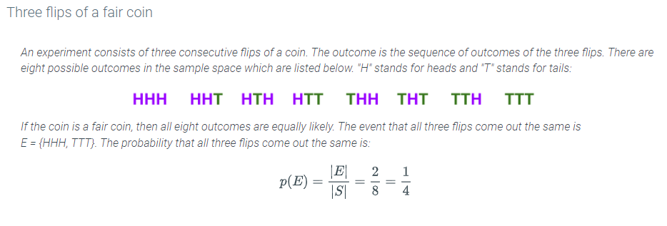
In this lesson you will be working with the probability of all possible outcomes. That might sound like a daunting task, but it’s not at all. Take a look at the experiment of rolling a six-sided fair die. There are six outcomes and each outcome has a probability of 1/6. If we add all those probabilities together, you get a sum of 1. As a percent value, 1 is 100%. The probability of getting either a 1, 2, 3, 4, 5, or 6 in this experiment is 100%.

Keep in mind, the sum of all the probabilities in a sample space should equal 1. If the sum is not 1, then something in the experiment is either unfair or there is a defect in the system.

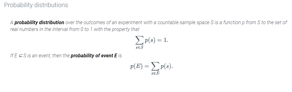
The focus of this lesson is probability distribution, which is this sum of probabilities. If all the probabilities for the event subsets are equal, then the distribution is known as a uniform probability distribution

Probability distributions

A natural question to ask about an experiment is: what is the likelihood (or probability) that a particular outcome occurs?

The uniform distribution

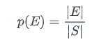
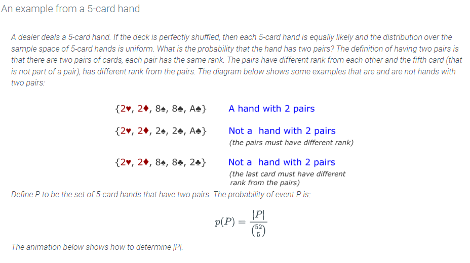
In many scenarios, the probability of every outcome in the sample space is the same. The probability distribution in which every outcome has the same probability is called the uniform distribution. Since there are |S| outcomes in sample space S and their probabilities sum to 1, under the uniform distribution, for each s ∈ S, p(s) = 1/|S|. The uniform distribution reduces questions about probabilities to questions about counting because for every event E,

Lesson summary

Now that you have completed this lesson you should be able to calculate the probability of an independent outcome or event. Take a moment to think about what you’ve learned in this lesson:

• A probability distribution is just the sum of each event subset’s probability. The sum of the distribution should always be 1 if the experiment is fair.
• If the probability of each element is the same, then this is a uniform distribution.
• Use this formula to calculate the probability of an event:
  Probability of an event=Number of Favorable OutcomesTotal Number of all Possible Outcomes

5.5 Lesson: Probability: Inclusion-exclusion rule

Lesson introduction

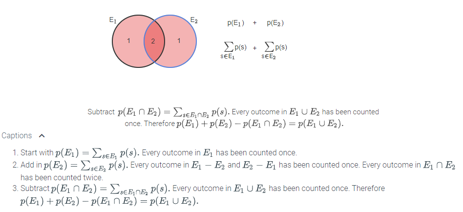
This lesson is going to seem very familiar. Remember using the inclusion-exclusion rule for counting sets? In this lesson you will use exactly the same principle in determining probabilities of events. Except in this lesson sets that are disjoint will be referred to as mutually exclusive-similar principle, new name.

Calculating probabilities for unions of events

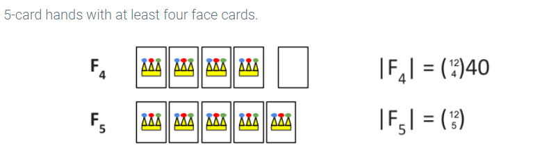
Sometimes it is easier to determine the probability of an event by defining the event in terms of other events. Suppose we would like to calculate the probability that a 5-card hand has at least four face cards (jack, queen, or king). It is easier to determine the probability that the 5-card hand has exactly four face cards or exactly five face cards. Adding the probabilities of the two events gives the correct answer because a hand can not have four face cards and five face cards at the same time.

Two events are mutually exclusive if the two events are disjoint (i.e., the intersection of the two events is empty). It follows from the definition of the probability of an event that if E₁ and E₂ are mutually exclusive, then:

Lesson summary

Now that you have completed this lesson you should be able to calculate the probability for mutually exclusive events using the inclusion-exclusion rule. Take a moment to think about what you’ve learned in this lesson:

• The probability of two events happening as an OR-that is, either this event A happens OR this event B happens-is a union of the event sets. If the two sets do not overlap, then they are referred to as exclusive.
• To calculate the probability of the union of two mutually exclusive events add the probability of each event.
• The inclusion-exclusion principle for counting (with two sets) is similar to the inclusion-exclusion principle in probability. If the event sets overlap, then you must subtract the probability of their intersection. To calculate the probability of two events that overlap, add the probability of each event then subtract the probability of the overlapping events.
• Here’s a quick example of the inclusion-exclusion principle in probability. If you were to try to calculate the probability of drawing a red card or a face card from a standard deck of cards, you need to take into account that some of the red cards are face cards (the events are not mutually exclusive). The calculation would look like this: p(red U face) = p(red) + p(face) – p(red face). The final answer would be:

5.6 Lesson: Probability: Complement rule

Lesson introduction

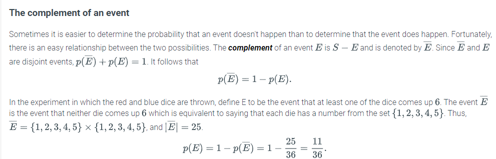
What if you wanted to know the probability of getting at least one tail when flipping a coin six times? The easiest way to get the answer is to consider the situation in the opposite view: “What is the probability of not getting even one tail?”

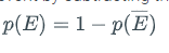
Just like when counting using the complement of a set, you can calculate the probability of an event by subtracting the probability of the event not happening from the probability of the event certainly happening (that is, 1 or 100%).

In case you are wondering, the probability of getting at least one tail in six coin flips is

The complement of an event

Sometimes it is easier to determine the probability that an event doesn’t happen than to determine that the event does happen. Fortunately, there is an easy relationship between the two possibilities. The complement of an event 

Lesson summary

Now that you have completed this lesson you should be able to calculate the probability of an event using the complement rule. Take a moment to think about what you’ve learned in this lesson:

• Using the idea of the complement of a set is very useful in calculating the probability of cumbersome events.
• Just like when counting using the complement of a set, you can calculate the probability of an event by subtracting the probability of the event not happening from the probability of the event certainly happening. Use the formula

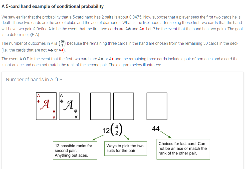
Lesson summary

Now that you have completed this lesson you should be able to determine if two events are independent or dependent. Take a moment to think about what you’ve learned in this lesson:

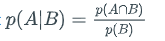
• Conditional probability is based on two events, A and B, which are dependent. If event B occurs first, the new probability (sample space for event A) has now changed. The probability for event A given that B occurred first is notated by (A|B) and is calculated using this formula: 

• Remember, just because you’re working with dependent events (or overlapping, intersecting sets), it does not mean all the concepts you have used for counting do not also apply for probability. For example, you can use the rules of complements of sets or events to help calculate the conditional probability.

5.9 Lesson: Independent vs. dependent events

Lesson introduction

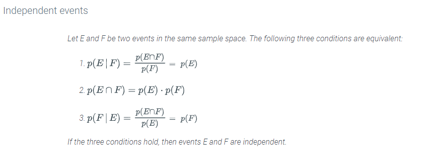
As you learned in a previous lesson, when two events are independent their order of occurrence doesn’t matter – neither event will influence the other. For example, if in your job you’re wondering whether one thing is having an effect on another, then determining that the probabilities of those “things” (events) are independent or not will help you find the solution.

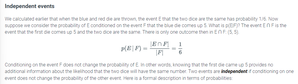
As you will learn in this lesson, you can use the following criteria to determine independence of two events:

• The conditional probabilities of both events equals the probability of the second event alone.
• The probability of the intersection of event sets is the same as the product (multiplication) of the individual probabilities.

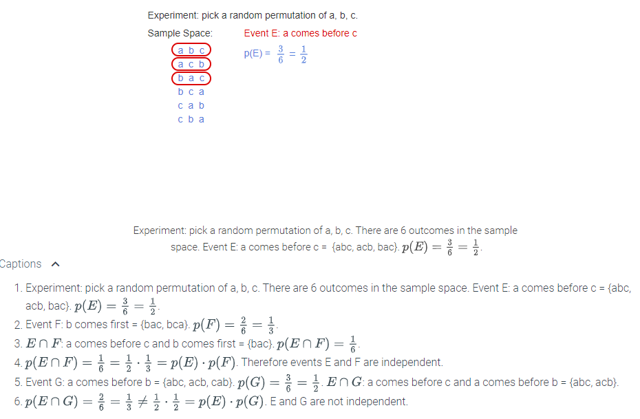
Independent events

Calculating the probabilities of two independent events

In some situations, it is reasonable to assume that two events are independent because it is unlikely that one event influences the other event. For example, if a single die is rolled twice, the event that the die comes up 5 on the first roll is unlikely to affect whether or not the die comes up 5 again on the second roll. If two events are independent, it is easier to calculate the probability that both events happen because the probability that both occur is the product of the probabilities that each event occurs. If X and Y are events in the same sample space, and X and Y are independent, then

p(X ∩ Y) = p(X) · p(Y)

Lesson summary

Now that you have completed this lesson you should be able to determine the conditional probability of dependent events. Take a moment to think about what you’ve learned in this lesson:

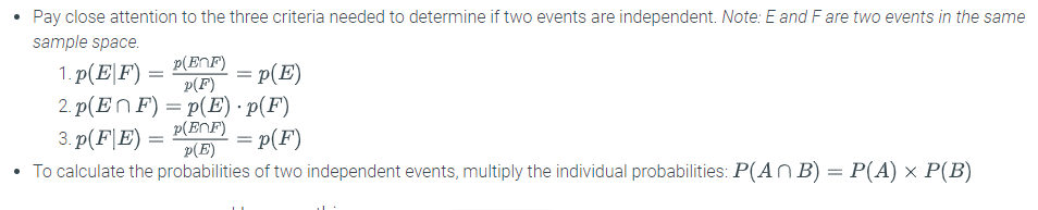
• Pay close attention to the three criteria needed to determine if two events are independent. Note: E and F are two events in the same sample space.

5.10 Lesson: Bayes’ Theorem

Lesson introduction

In computer science, machine learning and artificial intelligence are very common topics. If you are working with algorithms in machine learning, then you are creating algorithms which analyze data to help the machine “learn.” As part of that analysis you will need to know Bayes’ theorem.

Bayes’ theorem allows you to determine conditional probabilities of several events. It also allows for updates to the calculation based on observations of events, evidence, or even suppositions. Using this theorem you can update your probability calculations until you get a more accurate result.

For example, Bayesian updating is used in email spam filters to determine the likelihood (probability) an email is spam (unsolicited) or non-spam (solicited) using the words in the email. The algorithm “learns” to filter better and better as the programmer provides feedback in the form of observations on whether or not the email was really spam. The algorithm is then updated and becomes more accurate in the future.

Bayes’ Theorem

Suppose a gambler has two dice that look the same, except that one is a fair die and the other is loaded. When the fair die is rolled, each of the six outcomes is equally likely to occur. When the loaded die is rolled, a 6 is twice as likely to come up than the other outcomes. The probability distribution over the outcomes of the loaded die is:

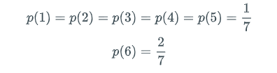
The gambler has both dice in her pocket and pulls out a random one for a game. Is it possible to reason about which die she picked based on the outcomes of the rolls? Presumably, if a 6 comes up more often than expected, it is more likely that the gambler is using the loaded die. Bayes’ Theorem provides a way to reason quantitatively about the likelihood that the die is loaded based on the evidence of the outcomes. Bayes’ Theorem is the cornerstone of many algorithms in machine learning in which the goal is to determine the likelihood of some event based on data obtained from observations.

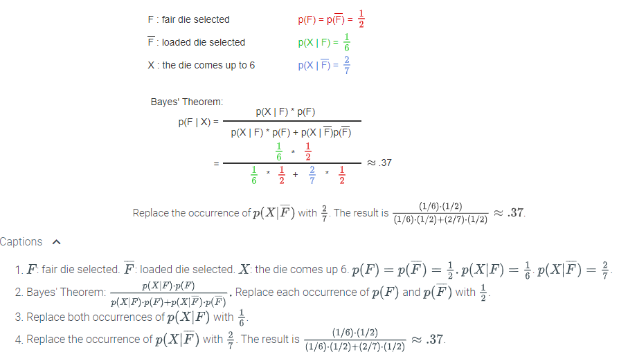
In the loaded die problem, the event F is the event that the gambler selects the fair die and F is the event that she selects the loaded die. Since she picks a die at random, p(F) = p(F) = 1/2. Let X be the event that the die comes up 6. We know the probability of X conditioned on F and F:

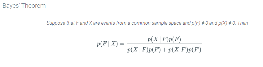
We would like to know the probability of F or F conditioned on observing a 6 (i.e. conditioned on the event X). Thus, we want to know p(F|X). Bayes’ Theorem provides a way to determine p(F|X) from p(X|F), p(X|F) and p(F):

Testing for defects in computer chip manufacturing

Suppose that 1 out of every 1000 computer chips produced by a chip manufacturer has a defect. The manufacturer has developed a method to test the chips, but the test is not perfect. If the chip has a defect, the test will discover the defect with probability 0.99. If the chip does not have a defect, the test will report that it does have a defect with probability 0.02. If the outcome of a particular test indicates that there is a defect, what is the likelihood that the chip is actually faulty?

Let D be the event that the chip has a defect. Let T be the event that the test outcome indicates a defect. Here is a summary of the probabilities given:

• p(D) = 0.001 because one out of every 1000 chips has a defect.
• p(T|D) = 0.99. If the chip is faulty, a test will indicate a defect with probability 0.99.
• p(T|D) = 0.02. If a chip does not have a defect, the test reports that it has a defect with probability 0.02.

Applying Bayes’ Theorem, we get:

Lesson summary

Now that you have completed this lesson you should be able to determine the conditional probability of a dependent event using Bayes’ theorem. Take a moment to think about what you’ve learned in this lesson:

• Bayes’ theorem, based on conditional probabilities, allows you to update the probability of hypotheses when provided evidence from observations.
• The formula for Bayes’ theorem states the relationship between p(H)-the probability of the hypothesis before the evidence, and P(H|E) the probability of the hypothesis after getting evidence: 

• Bayes’ theorem is very commonly used in determining the likelihood of “false-positives.” In other words, it is used to determine how likely a test or algorithm will produce an incorrect result. This theorem is important in factory applications (determining if the items being produced are defective or not), in medical testing (determining the accuracy of diagnostic tests), and many, many other computer science applications.

5.12 Lesson: Random variables

Lesson introduction

In this lesson you will be introduced to the concept of a random variable. It is a “variable” because it can take on different numerical values, but it’s called “random” because that numerical value is dependent on a random, experimental outcome.

Essentially, a random variable is a rule of association between each outcome of an experiment and some value defined by the rule. For example, as an experiment you randomly grab a pair of shoes in a shoe store to determine the probability of a specified outcome. A discrete random variable could have the possible outcome value of the shoe size, since it is a finite or countably infinite type of value. However, a continuous random variable could have the outcome value of the price of the shoes, technically an uncountably infinite type of value.

In computer science random variables are used in data analysis among other applications. The calculation of the probability of a random variable’s outcome is important in system optimizations and quality control. For example, if you were working for an airline you could use random variables to determine how many components failed to work in a random sample of 20 airline passengers, or the baggage weight of a sample of 30 airline passengers.

In this lesson you will calculate the values and ranges of random variables by applying the binomial theorem. If you need a refresher now is the time to go back to the “Binomial Theorem” lesson in Unit 4, Module 17.

Random variables

Many problems are concerned with a numerical value associated with the outcome of an experiment. For example, the rules of a game may depend on the sum of the values of a roll of two dice and not on the particular outcome of each individual die. In a random assignment of tasks to processors in a distributed network, the number of tasks assigned to a particular processor is likely to be an important factor in assessing the quality of the assignment. After a few days of observations of the stock market, the amount of money lost or gained is the quantity of interest. A random variable assigns a real number to every outcome of an experiment and therefore provides a way of targeting a particular quantity of interest.

Random variable

A random variable X is a function from the sample space S of an experiment to the real numbers. X(S) denotes the range of the function X.

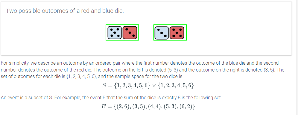
As an example, consider the experiment in which a red and blue die are rolled. Define the random variable D to be the sum of the two outcomes. The input to the function D is an outcome of the experiment which in the case of the dice is specified by a pair (x, y), where x is the number on the blue die and y is the number on the red die. Then D(x,y) = x + y. The diagram below shows two possible outcomes of the roll of the dice and the value of X for each outcome.

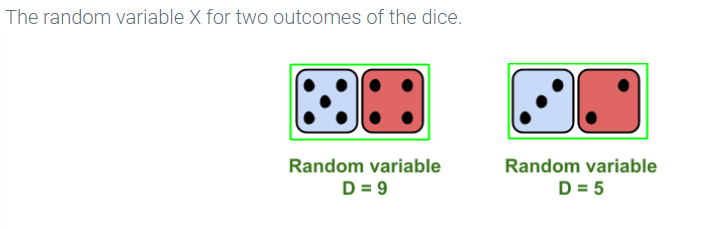
If X is a random variable defined on the sample space S of an experiment and r is a real number, then X = r is an event. The event X = r consists of all outcomes s in the sample space such that X(s) = r. p(X = r) is the sum of p(s) for all s such that X(s) = r.

Consider again random variable X defined to be the sum of the numbers on a blue and red die after they are thrown. The event that X = 4 is the set {(1,3),(2,2),(3,1)}, and p(X = 4) = 3/36 = 1/12.

Distribution over a random variable

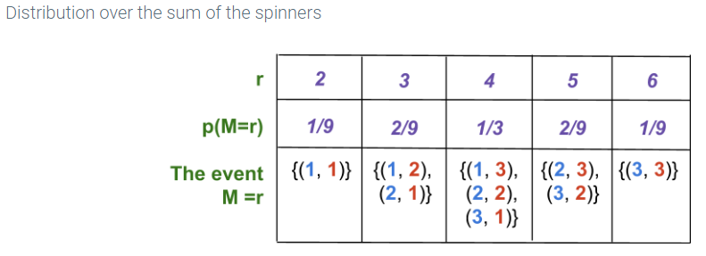
The distribution of a random variable is the set of all pairs (r, p(X = r)) such that r ∈ X(S)..

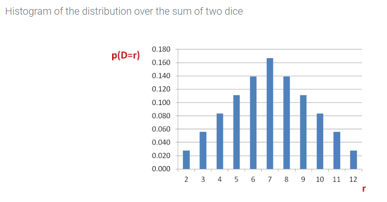
Since a random variable has some value for every outcome in the sample space, the sum of the values p(X = r), over all r ∈ X(S), must equal 1. For example, the probabilities from the animation above all sum to 1:

Lesson summary

Now that you have completed this lesson you should be able to determine the values and ranges of random variables. Take a moment to think about what you’ve learned in this lesson:

• A random variable is a rule of association between each outcome of an experiment and some value defined by the rule.
• There is a connection between random variable probability distribution and the binomial theorem you learned about in the “Binomial Theorem” lesson in Unit 4, Module 17.
• The probability of an event in a sample space is also the probability of the associated random variable value. Therefore, to calculate the probability distribution of a random variable, apply the same concepts as you did in the “Probability of an Event” lesson in Module 18.

5.13 Lesson: Expectation of a random variable

Lesson introduction

The concept of “expected value” at its core is just the value you would expect to have as an outcome of an experiment. Expected values are especially useful in determining whether games are fair or unfair. In particular, the popular games in Las Vegas each have an expected value which is unfair against the player. The game has to be set up this way, otherwise the Vegas casinos would not make any money.

Here’s a quick example of calculating expected value for a very simple game. The game involves rolling a single six-sided dice. If the player rolls a 3, they win $8. However, if they roll anything else, they only win $1. In order to play one round of the game, the player pays $4. To calculate the expected value of this game, create a probability distribution. Multiply each outcome, winning $8 or $1, by their respective probabilities and add the results. 1 × 5/6 + 8 × 1/6 = 2.17. The expected value for the game is $2.17.

Since it costs the player $4 just to roll the dice, then 2.17 – 4.00 = –1.83. This is a loss of $1.83 for the player for each round of the game. If the net expected value was zero, then the game would be “fair.” If the net expected value was positive, then the game would still be unfair—but in favor of the player (the house would lose money).

Expected or average value of a random variable

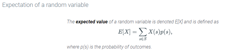
The distribution over a random variable provides a great deal of information about the outcome of the variable. The expected or average value of a random variable is a useful way to summarize the information in the distribution.

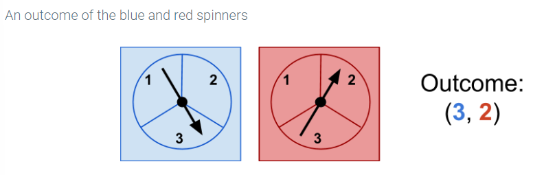
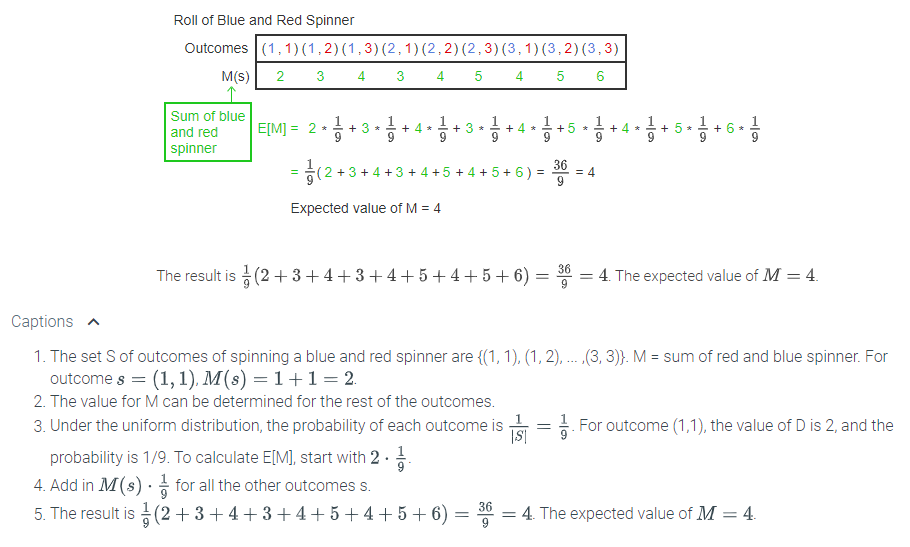
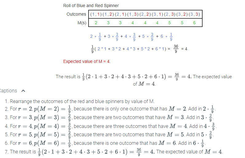
To illustrate expectations of a random variables, we consider an experiment in which a player in a game spins two spinners: a blue spinner and a red spinner. The outcome of each spinner is 1, 2, or 3. The outcome of the experiment is an ordered pair (x, y), where x is the outcome of the blue spinner and y is the outcome of the red spinner. Thus, the sample space of the experiment is {1, 2, 3} × {1, 2, 3}. The experiment is very similar to rolling two dice, but the sample space is smaller to keep the example simpler. Here is a picture of two outcomes of the spinner and the ordered pair representing the outcomes.

Expected winnings from a lottery

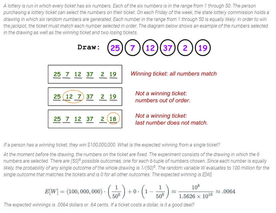
If the sample space is large, it can be tedious to add up the values of the random variable for each point in the sample space individually. The Theorem below gives a way to calculate the expectation of a random variable by grouping the outcomes according to the value of the random variable. There is a term in the sum for each value r in the range of X. The value of r is multiplied by the probability that the random variable X is equal to r.

An alternative way to calculate the expectation of a random variable

Lesson summary

Now that you have completed this lesson you should be able to calculate the expected value of a random variable. Take a moment to think about what you’ve learned in this lesson:

• To calculate expected value, create a probability distribution and multiply each outcome value by its probability, then add the results. If there is a cost to “play,” then the net expected value can be calculated by subtracting the cost from the expected value.
• Recall from your previous lesson, a random variable has values assigned from the outcomes of an experiment. Calculating the expected value of random variables is the same as described in the previous bullet-same principle, different name.

6.1 Unit 6: Modeling Computation

This is the beginning of Unit 6 in this Discrete Mathematics II course.

The material in this unit comprises 13% of the high-stakes assessment and includes such concepts as:

• Theory of computation
• Deterministic Finite State Automata (DFA)
• Nondeterministic Finite State Automata
• State diagrams and transition tables

Believe it or not, computer science is a fairly new discipline. One of its oldest areas of study is the theory of computation. Rather than using pen and paper, automata (machines) are used to model computation. There is no need to have big, powerful computers to model how calculations take place. Automata are simple concepts, but provide a framework to write effective algorithms, explore the correctness of those algorithms, or compare approaches to solving problems. In some cases automata also tell us if a problem can or cannot be solved.

Over the past few years the theory of computation has developed in many different directions and evolved in many exciting ways. Standard application of automata include pattern matching, syntax analysis, and software verification. In recent years, novel applications have emerged from biology, physics, cognitive sciences, neurosciences, linguistics, and other scientific domains. Developments in the information technologies warranted an increased need for formal designs and verification methods to ensure prescribed and secure performance of networks and mobile devices.

To ensure reliability of computing systems, software development methods need to include automatic verification that allows for the detection of defects. In game constructions automata are used to define the means of controlling a system and force it to satisfy a set of requirements in a given environment.

As you go through this module you will start recognizing automata in many forms—in the programs that you may have written, in the ways a programming language compiles code, or in operating elevators or a gum machine. Wherever rules and order of any kind are in place, these concepts can be used to formalize, define, or implement them.

6.2 Module 21: Deterministic Finite State Machine

This page marks the beginning of Module 21. This module contains six lessons:

• Theory of computation
• Introduction to deterministic finite state automata (DFA)
• DFA state diagrams
• DFA state transition tables
• Analyzing transition rules of a DFA
• Evaluating outcomes of a DFA

What do vending machines, traffic lights, speech recognition, video games, and natural language processing have in common? They are all applications of deterministic finite automata (i.e., machines), or DFAs, a theoretical concept of a computing machine. DFAs are models or theoretical concepts, not real computing machines. They explore ways computation could be carried out in efforts to provide blueprints of real automated artifacts or to learn how to build better actual machines or more efficient algorithms.

A DFA uses protocol analysis, text parsing, video game character behavior, security analysis, CPU control units, natural language processing, and speech recognition. Additionally, many simple (and not so simple) mechanical devices are frequently designed and implemented using DFAs, such as elevators, vending machines, and traffic-sensitive traffic lights. These machines take an input, process the input using internal logic that is defined by the various finite states the machine can be in and changes those states until the input is all processed out, i.e., all the letters of the input string are used up to guide the machine through the desired states.

DFAs are crucial to many areas, most notably text processing, compiling, and hardware design in the domain of computer science. They help us check, for example, if a line of code is syntactically correct, meaning that it adheres to the rules of the programming language.

MODULE OBJECTIVE: By the end of this module, you should be able to determine outcomes of the current or next state of a deterministic finite state machine.

6.3 Lesson: Theory of computation

Lesson introduction

Many problems have solutions, but some do not. We use a variety of computing machines to code the algorithms that solve problems. As you may remember from Unit 1: “Algorithms and Big-O Estimates,” when analyzing the solutions it is irrelevant how fast our actual computing system is or how much memory we have on the hard drive. We study, instead, how these algorithms perform on abstract computing devices called machines.

This lesson provides an introduction to the major families of automata, the theoretical models for computing machines, and their respective languages and grammar. These concepts directly influence uncountable domains of models in computer science, including developing software, understanding what we can expect from software, and understanding if we are able to write a program to solve a given problem or if we should try an alternative approach that will approximate the solution, or bet on chances.

Lesson objective

After completing this lesson you should be able to describe theoretical models for computing machines, the major families of automata, and the respective languages and grammars.

Introduction to computational models

Computation is any type of calculation that includes both arithmetical and non-arithmetical steps and follows steps that provide a solution to a problem. Computational models are abstract models that allow computer scientists to reason about what can and cannot be computed by a particular kind of device. Many computational models exist in the field of computer science, including pushdown automata, linear-bounded automata, and Turing machines.

Major families of automata

There are four major families of automaton listed in order of complexity from simplest to most complex.

The finite state machine is the simplest family of automaton. In a finite state machine, every bit exists in either of two states, 0 or 1, and a finite number of possible inputs exist. Finite state machines are ideal for small amounts of memory. Finite state machines are used for analysis of mathematical problems and to recognize regular languages. Finite state machines handle Type-3 grammars and regular languages.

A pushdown automaton uses a stack, or an abstract data type that collects elements. Pushdown automata are used in theories to determine what machines can compute. Pushdown automata handle Type-2 grammars and context-free languages.

A linear-bounded automaton consists of two endmarkers with input in between. Data is contained in a “tape” between the endmarkers. Linear-bounded automata handle Type-1 grammars and context-sensitive languages.

A Turing machine is the most complex family of automaton. The Turing machine consists of a finite automaton with infinite storage. The Turing machine can change symbols on its tape, and is thought to be able to model all computations that can be handled by modern computers. Turing machines handle Type-0 grammars and recursively enumerable languages.

Languages and grammars

We use language with a set of grammar rules to communicate among ourselves, and so do automata. Each family of automata have a specific languages and grammar. Noam Chomsky gave a mathematical model of grammar which is used for writing computer languages.

Language theory describes languages as sets of operations over an alphabet. Several classes of formal languages exist. The Chomsky hierarchy describes a series of language specifications in increasing levels of complexity. Each type of language corresponds to a class of automata that recognizes that language type. Formal languages are the preferred method for specifying problems that must be computed.

A computational model receives a string as input and produces an output based on the input. This material focuses on computing devices that output “yes” or “no”. If the computational model outputs “yes” in response to a particular input string, then the model accepts the string. If the model outputs “no” in response to a particular input string, then the model rejects the string. The language accepted by a computational model is the set of all strings which the computational model accepts.

An example of a language

An example of a language is the language consisting of all binary palindromes. A palindrome is a string that reads the same backwards and forwards. Thus, elements of this language include strings such as 0, 000, 111, 10101, and 1100011. The string 0101 would not be an element of this language.

A grammar is a set of rules for generating strings. The language generated by a grammar is the set of all strings that can be generated according to the rules of the grammar.

The finite state automaton

An important computational model, and the focus of the remainder of this unit, is the finite state automaton. A finite state automaton (plural: finite state automata) consists of a finite set of states with transitions between the states triggered by different input actions. Finite state machines are used in many computer science applications. Most of this section’s examples show how finite state automata can model logical devices. Finite state automata are also used in specifying network and communication protocols, compiler design, and text search. A finite state automaton is also known as a finite state machine (FSM).

Lesson summary

Now that you have completed this lesson you should be able to describe theoretical models for computing machines, the major families of automata, and the respective languages and grammars. Take a moment to think about what you’ve learned in this lesson:

• Computation is the process of solving problems using a physical device. The physical device that can perform computations is referred to as a “computer.”
• Computational models are abstract models that allow computer scientists to reason out what can and what cannot be computed.
• Computational models receive a string as an input and produce an output based on the input. Some models output “yes” when the input string is accepted by the machine or “no” if it is rejected.
• The set of strings accepted by a machine is called a language. A language is generated by a set of rules called grammar. The concepts of languages, grammars, and automata are intrinsically connected. A grammar generates a language that is accepted by an automaton.
• Finite state automaton is a computational model that consists of a finite set of states with transitions between the states triggered by different input actions. It is also called a finite state machine (FSM).

6.4 Lesson: Deterministic finite state automata (DFA)

Lesson introduction

In the previous lesson you were introduced to the term “finite state machines (FSM).” In this lesson you will learn about a specific category of FSM: deterministic finite state automata (DFA). Deterministic machines, when in an initial, predefined state, take a string as an input and change the machines’ states. They do this by processing the string by looking at its symbols starting from the beginning, the leftmost symbol of the input string. Regardless of what the automaton currently “sees,” (i.e., the position of the input string it is processing) there is no ambiguity about what it will do next. In deterministic automata, the next step of the automaton is defined by the current state and the letter or letters the automation is currently reading. There is no possibility of going into two different states at any given step, which is what makes it “deterministic.”

As you learned in the previous lesson, it is “finite,” not because it is completed in finite number of steps, but because it may have a finite number of states in which it could be found. As the DFA reads each symbol from the beginning of the input string it jumps states accordingly. It stops jumping between states when there is nothing more to process. If the end state of the automation is an “acceptable” state, then this automation accepts the input string; otherwise the input string is rejected.

The deterministic finite automata are the simplest models of computation; the regular languages they accept are the simplest of all formal languages and the grammars that generate them are the simplest of all grammars studied by the theory of computation.

Lesson objective

After completing this lesson you should be able to describe deterministic finite automata, regular languages, and regular grammars.

Deterministic finite automata

To determine whether a string is accepted or rejected, a finite state automaton processes the string one input symbol at a time and moves between states with each new symbol received. A deterministic finite automaton (DFA) is a finite state automaton whose next state is uniquely determined by the current state and the next input symbol.

DFAs are the simplest of the models of computation. DFAs are used for analysis of mathematical problems and to recognize regular languages. DFAs handle Type-3 grammars, the simplest of all grammars, and regular languages, the simplest of all formal languages.

A subway turnstile is an example of a DFA.

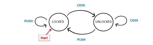
A DFA contains several components.

• A finite number of states that the automaton enters during the processing of a string.
• The alphabet, or a finite set of possible input symbols in a string.
• A transition function, which is a set of rules that determine the next state entered by the automaton based on the current state and the next input symbol received.
• A start state at which the processing of a string begins.
• One or more accepting states that represent the acceptance of a string if the automaton ends up in one of those states at the end of processing the string. A string is rejected if the automaton ends up in a non-accepting state at the end of processing the string.

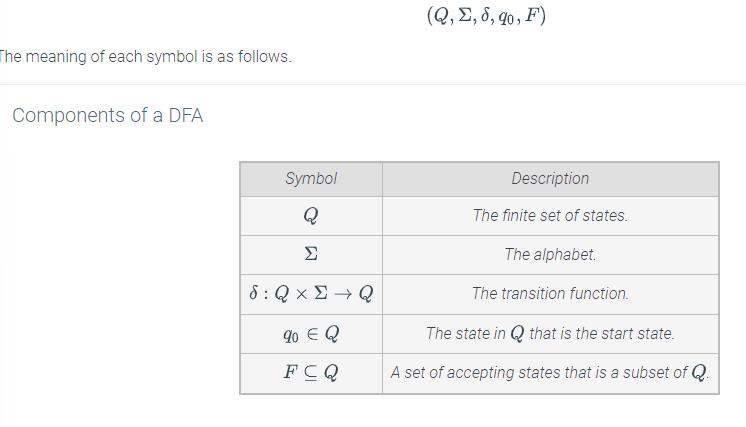
Formally, a DFA is defined using the following 5-tuple (quintuple), or ordered list of 5 elements.

Lesson summary

Now that you have completed this lesson you should be able to describe deterministic finite automata, regular languages, and regular grammars. Take a moment to think about what you’ve learned in this lesson:

• A deterministic finite automaton (DFA) is a finite state automaton whose next state is uniquely determined by the current state and the next input symbol.
• A deterministic finite automaton is a quintuplet (5-tuple) that consists of:
  • a set of states,
  • a set of symbols (alphabet),
  • a transition function (set of rules for transitioning between states),
  • an initial state, and
  • a set of final, accepting states.
• Initially the DFA is in the given initial state. It initiates its transitions by looking at the first symbol of the input string. The state the DFA will transition to depends on the symbol currently at the beginning of the input string and the transition function.
• A string is accepted by a DFA if the machine does not have any symbols from the initial string to read and it has transitioned into an accepting state.

6.5 Lesson: DFA state diagrams

Lesson introduction

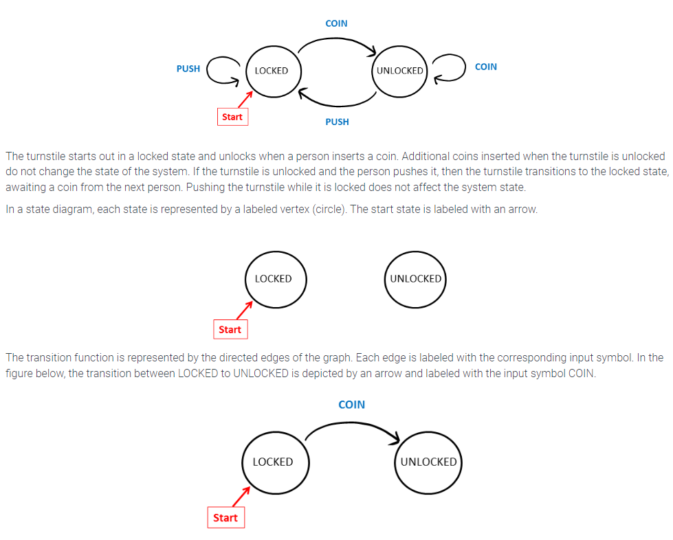
The behavior of DFAs is easily visually traced using their graphical representations, or state diagrams. The diagrams use circles to denote state, labeled arrows to denote the transitions (the rules of behavior of the DFA), and a special label that denotes the single start (initial) state. The states are often labeled to identify the final states of the DFA.

These state diagrams explain what happens with the automaton when it is in any of its states and when it encounters an alphabet symbol at the beginning of the unprocessed part of the input string. Every state has labeled arrows that come out of it, each labeled with one of the alphabet symbols. That way, the automata knows which state to transition to as long as there are letters in the input string. Once the letters from the input string are all used up for transitions, the DFA stops. If it stops in a final state, then the input is accepted.

Lesson objective

At the end of this lesson you should be able to interpret the graphical representation of a deterministic finite automata.

State diagrams

Previously, a subway turnstile was described as a DFA, with the states, alphabet, and transition function described in words. A DFA can be described more intuitively as a state diagram. A state diagram is a directed graph whose nodes represent states.

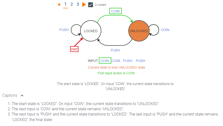
The following state diagram represents the behavior of the subway turnstile.

Lesson summary

Now that you have completed this lesson you should be able to interpret the graphical representation of a deterministic finite automata. Take a moment to think about what you’ve learned in this lesson:

• A state diagram is a visual representation of a deterministic finite automation.
  • Circles denote the states of the automation
  • The labeled arrows explain the transitions between states, i.e. they model the transition function.
• The automaton transitions between states jumping from one state to another following the arrow that is labeled by the next alphabet symbol from the input string.

6.6 Lesson: DFA state transition tables

Lesson introduction

Imagine playing Monopoly. You start the game at the Go square and move about using the rules of the game. Depending on the input from the dice, you move your character around the board. Each square on the board is associated with a set of rules defined by the game. The number on the dice is the input and the current square you are on, with all of the game rules that apply to it, is the current state of the game. When these rules are clearly defined, a machine can play the game on its own, automatically, or act as an automaton.

In the previous lesson you learned about state diagrams, but there is another format that can describe the transition functions: state tables. Instead of diagrams, the transition function can be described in a tabular format. State tables (state transition tables) give the next state of the automaton based on the current state and the symbol at the beginning of the input string. It has a row of states and a column of alphabet symbols. The matrix columns and rows define the states in which the automaton transitions to when in a given state, and the automaton reads the respective input symbol.

Lesson objective

After completing this lesson you should be able to interpret the internal states of a deterministic finite automata represented with state transition tables.

DFA state transition tables

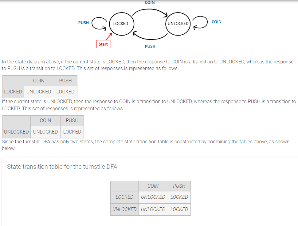
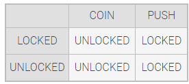
In addition to a state diagram, the transition function of a DFA can also be represented with a state transition table. In a state transition table, the rows represent the current state and the columns represent the possible input symbols. Each entry of the table indicates the next state for each current state and input symbol combination.

A state table can be constructed from a state diagram by analyzing the outcomes of each input symbol on each possible current state. The turnstile DFA is again shown below.

Lesson summary

Now that you have completed this lesson you should be able to interpret the internal states of a deterministic finite automata represented with state transition tables. Take a moment to think about what you’ve learned in this lesson:

• The transition function of a deterministic automation can be represented by a table that defines the state to which the automation transitions, based on the current state. The current states are represented as rows and the current alphabet symbols are represented in the columns of the state transition table.

• DFA transition functions can be described using words, state transition diagrams, or state transition tables, among other methods

6.7 Lesson: DFA analyzing transition rules

Lesson introduction

In the previous lesson you learned how to interpret the state transition table and in this lesson you will learn how to analyze the transitional rules.

As the DFA transitions to each state, it constructs an output string (or sentence). At each transition, the DFA concatenates another symbol or word to the output string or sentence. Once the DFA completes its transitions this output string or sequence is the output from DFA for the given input string. When all symbols from the input string are used up—that is, all transitions are complete—the DFA presents a complete output.

Lesson objective

After completing this lesson you should be able to analyze transition rules of a computational model for a deterministic finite automata.

Following the transitions of a DFA

When a DFA reads a string, the DFA begins at the start state and reacts based on the first symbol in the string. The process is repeated with subsequent symbols in the string until the end of the string is reached. The transition rules of a DFA can be analyzed using the state diagram or the state table of the DFA.

Lesson summary

Now that you have completed this lesson you should be able to analyze transition rules of a computational model for a deterministic finite automata. Take a moment to think about what you’ve learned in this lesson:

• The DFA always starts in the “start” state and initiates the transition based on the first symbol of the input string. In the new state it reacts to the second symbol, transitions to a new state, and so on.
• Some DFAs can build output as they transition based on the input symbol.
• The input and output alphabets may coincide, but they do not need to. The DFA with output is virtually a rewriting system, one that uses one string and generates another based on the rewriting rules defined by the transition function.

6.8 Lesson: DFA evaluating outcomes

Lesson introduction

DFAs, in the traditional theoretical context, accept or reject an input string. In other words, they recognize a language. They complete the transitioning based on an input string from the given language in a finite state; if an input is used up in the transitions and the automation is in a state that is not finite, then the string is not accepted, i.e., it does not belong to the language the automaton recognizes.

The DFA does not have a “long memory.” All a DFA “is aware of” is its current state and the symbol at the front of the input string. Therefore, there are languages the DFA cannot accept.

Lesson objective

After completing this lesson you should be able to determine the outcome of a given state based on the computational model or associated state transition table of a deterministic finite automata.

Finite state machines with output

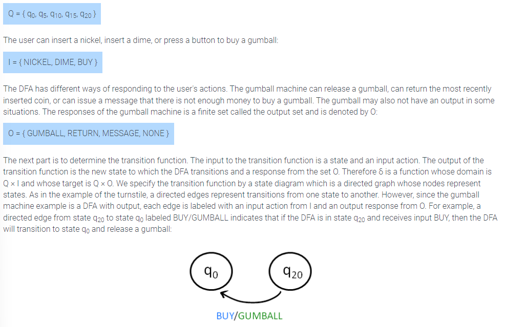
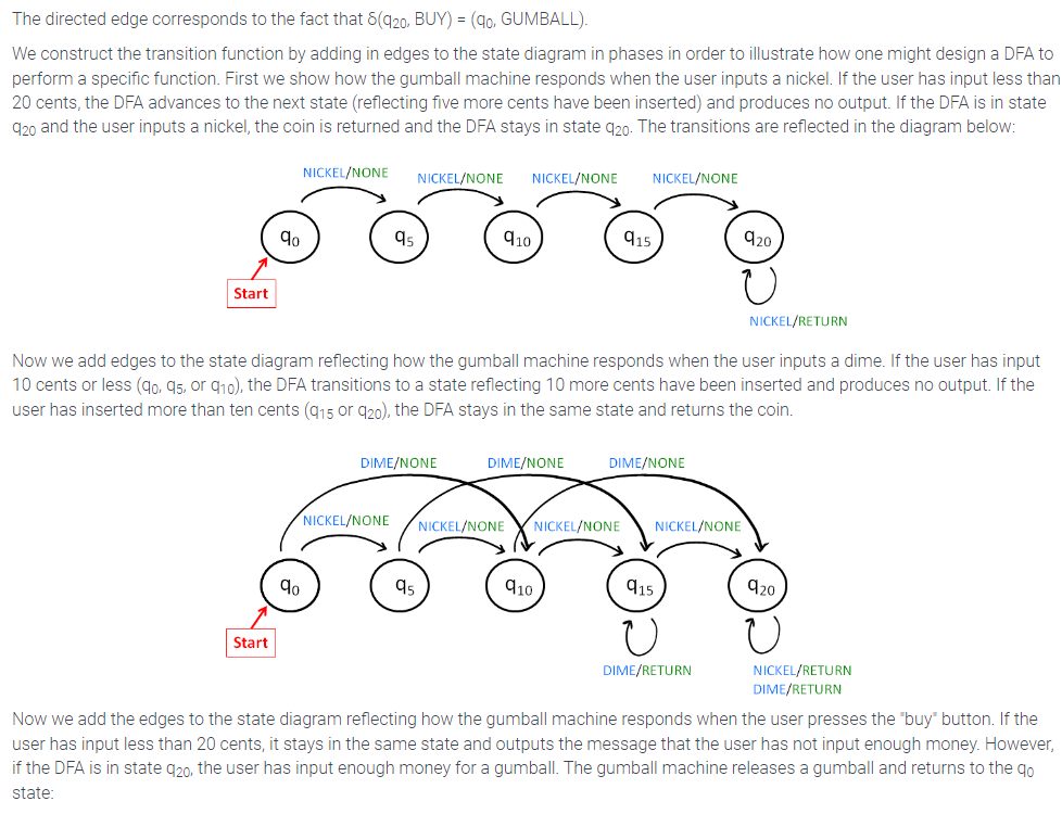
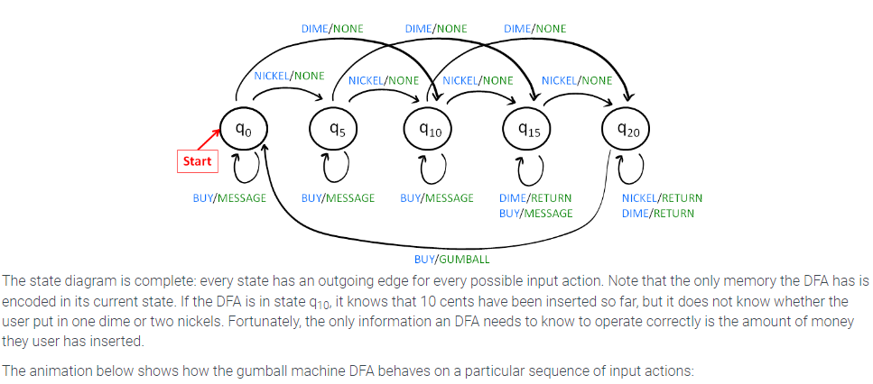
In the turnstile example, the response of the DFA was entirely expressed in the state, i.e., whether the turnstile is locked or unlocked. In some applications, a more detailed response is required. A deterministic finite automaton with output, or DFA with output, produces a response that depends on the current state as well as the most recently received input. We illustrate an DFA with output using an example of a gumball machine. The machine sells gumballs for 20 cents and accepts only nickels and dimes. To keep the example simple, the machine will not make change. If the user has already inserted 15 cents and then inserts a dime, the machine just returns the dime and remains in the same state. Five states represent the amount of money that has been inserted so far

DFAs that recognize properties

DFAs can also be used to determine whether an input string has a particular property. Instead of having input actions from a user, each input is a character from a finite alphabet. The sequence of inputs is a string over the input alphabet. An input string is accepted if the DFA ends up in an accepting state after each character in the string is processed. The set of all accepting states is a designated subset of the states.

Consider a DFA with input alphabet {0, 1}. There are two states: {ODD, EVEN}. The state EVEN is the start state and the state ODD is the only accepting state. The transition function for the DFA is specified by the state diagram below. As before, the start state is denoted by an arrow. The accepting state is shown with a double outline.

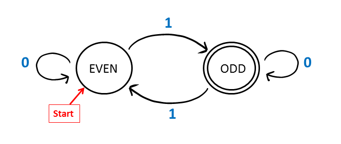
The DFA shown above accepts a binary string if and only if the number of 1’s in the string is odd. The property of whether a number is odd or even is called the parity of a number. The parity of a string is the parity of the number of 1’s. The state encodes whether the number of 1’s seen so far is odd or even. An input of 0 causes the DFA to stay in the same state. An input of 1 causes the DFA to change states.

Here is an animation of the action of the DFA on a particular input:

Recognizing valid passwords

In another example, consider a computer system that accepts a password composed of digits and letters of any length. A valid password must begin with a letter and have at least one digit. We will show a DFA that accepts an input string if and only if it is a valid password. The input alphabet is {D, L} which stand for “digit” and “letter”. There are four states: {START, INVALID, VALID, UNDECIDED}. The only accepting state is the VALID state. The state diagram for the DFA is given below:

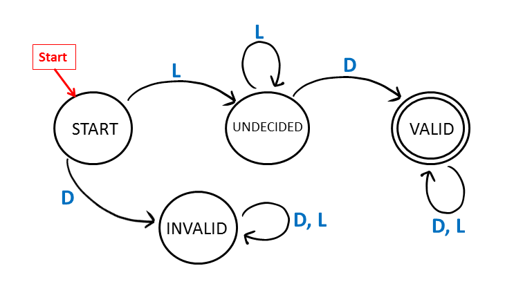
Note that if the first input character is a digit, the DFA will transition to the INVALID state because the first character is required to be a letter. If the DFA reaches the invalid state, the DFA will not accept the input regardless of what follows. On the other hand, if the first input character is a letter, the DFA will reach the UNDECIDED state. In the UNDECIDED state, the DFA is waiting to see if the input string contains a digit. If the DFA is in the UNDECIDED state and a digit appears, then all the conditions for the password have been met and the DFA will transition to the VALID state and will accept the input string regardless of what other characters follow. On the other hand, if the string ends while the DFA is in the UNDECIDED state (i.e., without having seen a digit in the input string), the DFA will not accept.

Lesson summary

Now that you have completed this lesson you should be able to determine the outcome of a given state based on the computational model or associated state transition table of a deterministic finite automata. Take a moment to think about what you’ve learned in this lesson:

• The finite states of a DFA is denoted by a doubled circle in the state transition diagram.
• An input string is accepted if the input string resulted in a DFA that is in a finite state.
• There are languages a DFA cannot recognize, as its memory is limited on the current state and the next symbol of the input string.

6.9 Module 22: Nondeterministic Finite State Machine

This page marks the beginning of Module 22. This module contains five lessons:

• Introduction to nondeterministic finite automata (NFA)
• NFA state diagrams
• NFA state tables
• NFA analyzing transition rules
• NFA evaluating outcomes

In the previous module you learned about DFAs. In this module you will learn about nondeterministic finite automata (NFA). DFAs can transition to one, and only one, state using a given input. Nondeterministic finite automata (NFAs) can transition to multiple states with one symbol, or even transition to another state without needing a symbol. DFAs and NFAs are equivalent (we will not go deep into the establishing of this equivalency), but for every DFA we can construct an NFA that will accept the same language and vice versa. We will look at the NFAs as automata that have less stringent constraints on the transition rules. This flexibility allows the NFA to serve a more appropriate and intuitive computational model, and model and describe processes or systems in a way that is easier to understand.

MODULE OBJECTIVE: By the end of this module, you should be able to determine outcomes of the current or next state of a nondeterministic finite state machine.

6.10 Lesson: Nondeterministic finite automata (NFA)

Lesson introduction

Unlike deterministic finite automata where the next state of the machine is uniquely determined by the state and the next symbol of the input string, in nondeterministic automata, one string could transition the machine to several states with or without input symbols. In that sense, every deterministic finite automaton is a nondeterministic one, but the reverse does not hold. The NDA are a superset of the DFAs. Just as before, an input string is accepted if there is a sequence of transitions that can arrive to a finite state from the input state using the string.

Lesson objective

After completing this lesson you should be able to compare deterministic finite automata to nondeterministic finite automata.

Non-deterministic finite automata

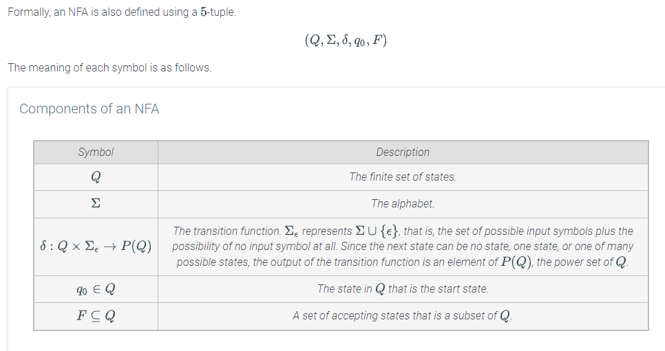
A non-deterministic finite automaton (NFA) is a finite state automaton whose next state is not uniquely determined by the current state and the next input symbol. In contrast to a DFA, in which the current state and the next input symbol uniquely determine the next state, an NFA can have more than one possible state (or no state at all) to which the NFA can transition given the current state and the next input symbol. In addition, an NFA can have transitions from one state to another without reading in an input symbol at all, a transition known as an epsilon transition and represented by the symbol �.

Similar to a DFA, an NFA contains several components.

• A finite number of states that the automaton enters during the processing of a string.
• The alphabet.
• The transition function. In an NFA, an input symbol, or no input, can cause a transition to the next state. Because the next state of an NFA can be no state, one unique state, or one of many possible states, the output of the transition function is an element of �(�), the power set of �, or the set of all subsets of �.
• The start state.
• One or more accepting states.

Lesson summary

Now that you have completed this lesson you should be able to compare deterministic finite automata to nondeterministic finite automata. Take a moment to think about what you’ve learned in this lesson:

• Nondeterministic finite automata are a quintuplet, where the transition function maps into the power state of the set of states. The components of the NFAs are the states set, the alphabet, set of final states, initial state, and a transition function.
• NFAs can transition into multiple states with one symbol or no symbols.
• An epsilon transition is a transition from one state or another without reading an input symbol.

6.11 Lesson: NFA state diagrams

Lesson introduction

Similar to a DFA, the NFA transition functions can be represented via state transition diagrams. The transitions for which no input symbol is used are labeled with the epsilon symbol. Pay attention to the similarities and differences between the state diagrams of an NFA and DFA.

Lesson objective

After completing this lesson you should be able to interpret the graphical representation of a nondeterministic finite automata.

NFA state diagrams

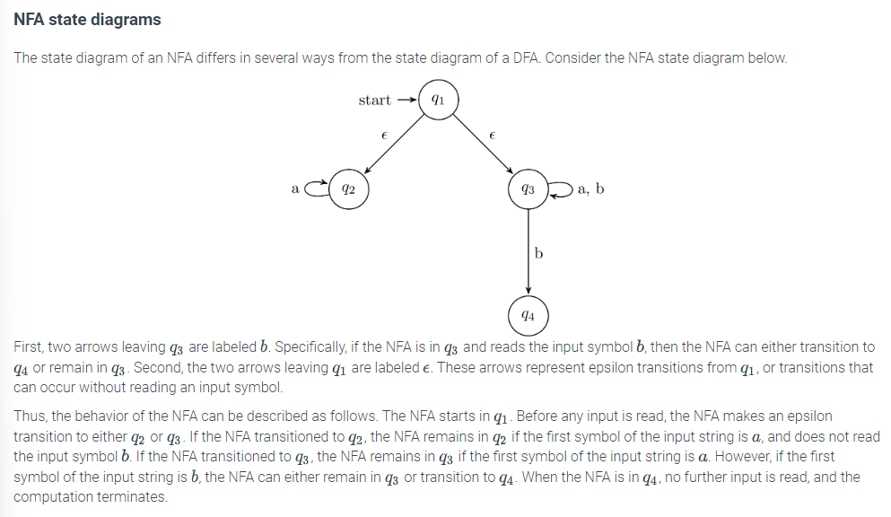
The state diagram of an NFA differs in several ways from the state diagram of a DFA. Consider the NFA state diagram below.

6.12 Lesson: NFA state transition tables

Lesson introduction

Just like with DFAs, instead of diagrams, the NFA’s transition functions can be presented in a tabular format. State tables, or state transition tables, give the next state of the automaton based on the current state and the symbol at the beginning of the input string or without a symbol. It has a row of states and columns of alphabet symbols including the epsilon symbol, which denotes triggering a transition without reading a symbol from the input string. The matrix of columns and rows includes states that the automaton transitions to. Based on the current state, the automaton reads the respective input symbol or transitions without using a symbol from the input string.

Lesson objective

After completing this lesson you should be able to interpret the internal states represented with state tables of a nondeterministic finite automata.

NFA state transition tables

Like DFA state tables, NFA state tables can be constructed from state diagrams, except a column corresponding to epsilon transitions should be added. Consider the state diagram below.

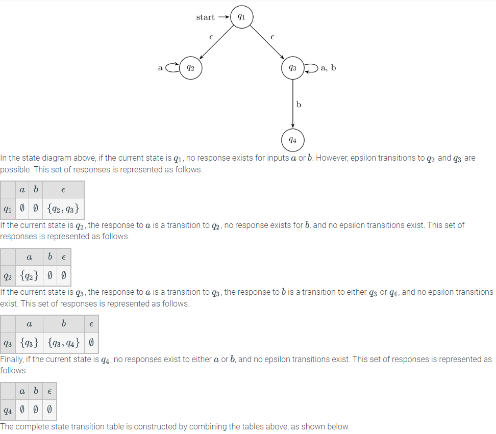
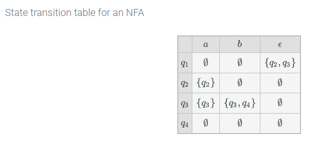
Lesson summary

Now that you have completed this lesson you should be able to interpret the internal states represented with state tables of a nondeterministic finite automata. Take a moment to think about what you’ve learned in this lesson:

• The transition function of a nondeterministic finite automation (NFA) can be represented by a table that defines the state to which the automation transitions, based on the current state (represented as rows) and the current symbol (represented in the columns of the state transition table), including the epsilon symbol which denotes transitioning without using a symbol from the input.
• NFAs’ transition functions can be described using words, state transition diagrams, or state transition tables, among other methods.

6.13 Lesson: NFA analyzing transition rules

Lesson introduction

Unlike DFAs, NFAs can end up in different states by either using input symbols or not using input symbols. Examining all possible sequences of actions provide insights into the language the NFA accepts.

Lesson objective

After completing this lesson you should be able to analyze state transition rules of a computational model of a nondeterministic finite automata.

Possible states of an NFA after computation

An NFA can take more than one possible action given the current state and the next input symbol. In determining the transitions of a non-deterministic finite automaton, all the possible sequences of actions given an input string must be considered.

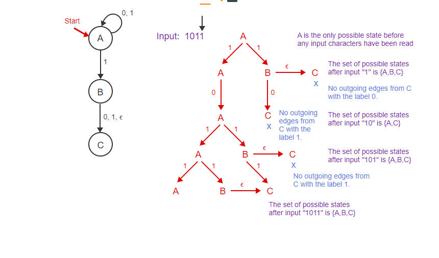
There is an � transition from B to C. There are no transitions out of C labeled 1. The set of possible states after input “1011” is {A,B,C}.keyboard_arrow_upCaptions

1. The start state of the NFA is A, and there are no � transitions out of A, so A is the only possible state before any input is read. The input string is 1011.
2. The first character of the input is 1. There are transitions from state A labeled with 1 to states A and B. Therefore, A and B are possible states after input “1&”.
3. There is an �-transition from B to C. Therefore C is also a possible state after input “1”. The set of all possible states after input “1” is {A, B, C}.
4. The next input character is 0. There is one transition labeled 0 out of state A which leads back to state A. Therefore A is a possible state after input “10”.
5. There is a transition labeled 0 out of B which leads to C. Therefore C is a possible state after input “10”. There are no transitions out of C after input “1”. The set of possible states after input “10” is {A, C}.
6. The next input character is 1. There are transitions out of A labeled 1 that lead to states A and B. A and B are possible states after input “101”.
7. There is an �-transition from B to C. Therefore C is also a possible state after input “101”.
8. There are no transitions out of state C labeled with 1. The set of all possible states after input “101” is {A, B, C}.
9. The next input symbol is 1. There are transitions from A to A and B. There is a transition from B to C.
10. There is an � transition from B to C. There are no transitions out of C labeled 1. The set of possible states after input “1011” is {A,B,C}.

Lesson summary

Now that you have completed this lesson you should be able to analyze state transition rules of a computational model of a nondeterministic finite automata. Take a moment to think about what you’ve learned in this lesson:

• Unlike DFAs, NFAs can end up in different states.
• When determining the transitions of a nondeterministic finite automaton, all the possible sequences of actions given in an input string must be considered.
• Starting with the initial state, follow the computations of the NFA to arrive to all possible states of an NFA after computation.

6.14 Lesson: NFA evaluating outcomes

Lesson introduction

An input string is accepted by an NFA if there is a sequence of transitions triggered by input symbols or no symbols that results in the machine reaching a final state. Due to the nondeterministic nature of the transitions, an extensive examination of all possible states of the NFA after calculation is needed to determine if an input string is accepted by the automation.

Lesson objective

After completing this lesson you should be able to determine the outcome of a given state based on the computational model and associated state transition table of a nondeterministic finite automata.

Accepting states of an NFA

An NFA may have more than one valid sequence of transitions for a given input string. Some sequences of transitions may lead to a dead end in which there are no transitions out of the current state labeled with the next input symbol. Some sequences of transitions may lead to a non-accepting state at the input string. An NFA accepts a string as long as at least one valid sequence of transitions corresponding to the input symbols exists that puts the NFA in an accepting state at the end of the input string. This concept is illustrated in the following animation.

Lesson summary

Now that you have completed this lesson you should be able to determine the outcome of a given state based on the computational model and associated state transition table of a nondeterministic finite automata. Take a moment to think about what you’ve learned in this lesson:

• An NFA may have more than one valid sequence of transitions for a given input string.
• Some sequences of transitions may lead to a dead end. Other sequences may lead to a non- accepting state at the input string.
• An NFA accepts a string as long as at least one valid sequence of transitions corresponding to the input symbols exists, putting the NFA in an accepting state at the end of the input string.