3.1 Unit 3: Recursion and Induction (21 Units)

This is the beginning of Unit 3 in this Discrete Mathematics II course.

The material in this unit comprises 20% of the high-stakes assessment and includes such concepts as:

• Recurrence Relations
• Induction Methods
• Summations and Limits
• Recursive Structures
• Recursive rules with functions, sets, and binary trees
• Simple Recurrence Relations

3.2 Module 9: Recurrence Relations

This page marks the beginning of Module 9. This module contains two lessons:

• Introduction to recursive relations
• Evaluating recursive relations

Recurrence notation

Recursion is a method that finds new values using previous values. 

Recurrence relations

A recurrence relation is an equation that expresses a new term using previous terms. To write the equation you need two pieces of information: the initial terms and a rule defining the new term based on the previous term.

Lesson summary

Now that you have completed this lesson you should be able to identify a recurrence relation. Take a moment to think about what you’ve learned in this lesson:

• Recursion is a method that finds new values using previous values.

3.4 Lesson: Evaluating a recursive relation

Lesson introduction

To paint a rectangle with a length of 2 feet and a width of 1 foot, you need 1×2=2 square feet of paint. Double the width to 2 feet, and you need 2×2=4 square feet. 

Recurrence relations

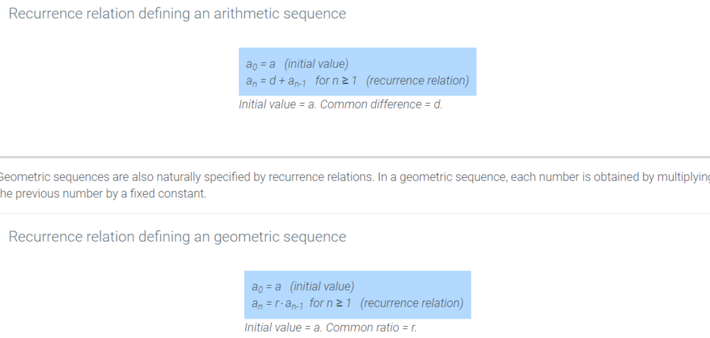
Some sequences are most naturally defined by specifying one or more initial terms and then giving a rule for determining subsequent terms from earlier terms in the sequence. A rule that defines a term a_n as a function of previous terms in the sequence is called a recurrence relation. For example, in an arithmetic sequence, each number is obtained by adding a fixed value to the previous number.

The Fibonacci sequence

Leonardo Fibonacci, a prominent mathematician in the middle ages, used a recurrence relation to define a sequence that is now known as the Fibonacci sequence. Fibonacci defined the sequence in an attempt to mathematically describe the population growth of rabbits.

Lesson summary

Now that you have completed this lesson you should be able to find terms in recursive geometric and arithmetic sequences. Take a moment to think about what you’ve learned in this lesson:

3.5 Module 10: Induction Methods

This page marks the beginning of Module 10. This module contains eight lessons:

• Computing summations
• Summation: limits and variables
• Inductive proof
• Divisibility proof by induction
• Induction proof of a recurrence relation
• Induction proof of closed summation
• Strong induction
• Well-ordering principle

3.6 Lesson: Summations

Lesson introduction

In the previous course you learned about finite and infinite series, including the concept of summations and sequences. This concept of summation is also relevant to the study of recursion relations. 

The summation of sequences (also called series) are one of the powerful tools in mathematics and computer science because they are necessary for the approximations and evaluations of functions.

Summation, sequences

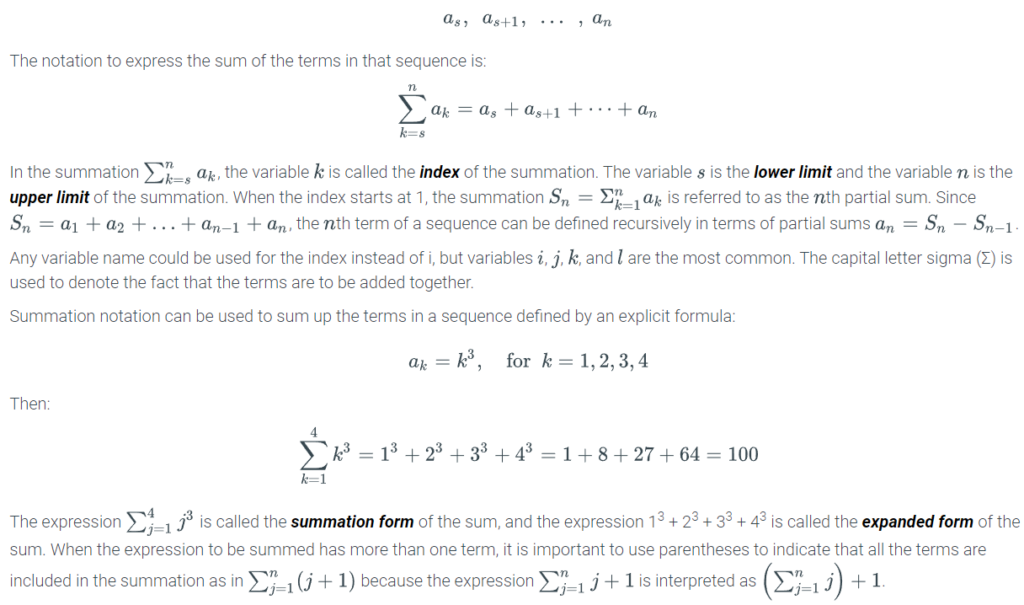
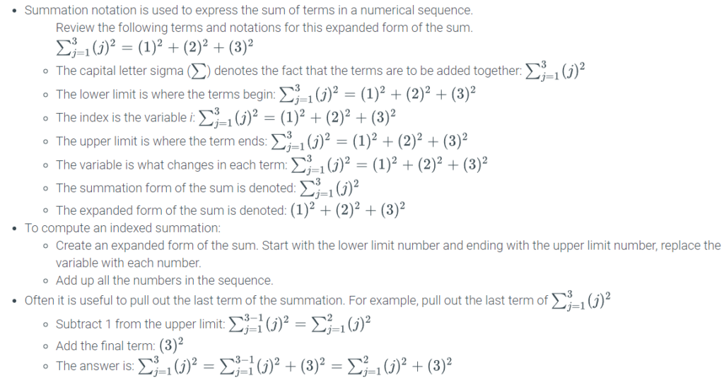
Summation notation is used to express the sum of terms in a numerical sequence. Consider a sequence:

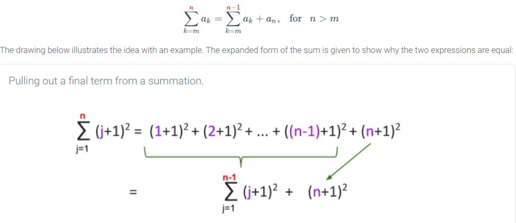
Pulling out a final term from a summation

In working with summations, it is often useful to pull out or add in a final term to a summation:

Lesson summary

Now that you have completed this lesson you should be able to compute sums of sequences written in summation or sigma notation. Take a moment to think about what you’ve learned in this lesson:

• Summation notation is used to express the sum of terms in a numerical sequence.

3.7 Lesson: Summation: limits and variables

Lesson introduction

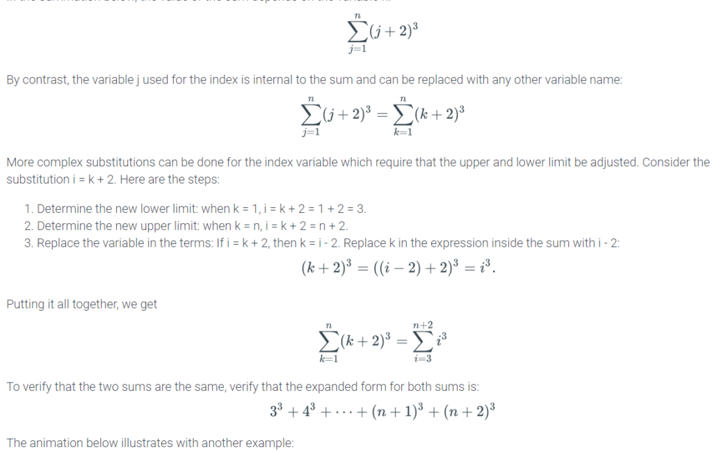
One of the key advantages of our new notation is the flexibility we gain to rewrite summations in equivalent forms. 

Change of variables in summations

When a variable is used to denote the lower or upper limit of a sum, the value of the variable must be provided in order to evaluate the sum. In the summation below, the value of the sum depends on the variable n:

Closed forms for sums

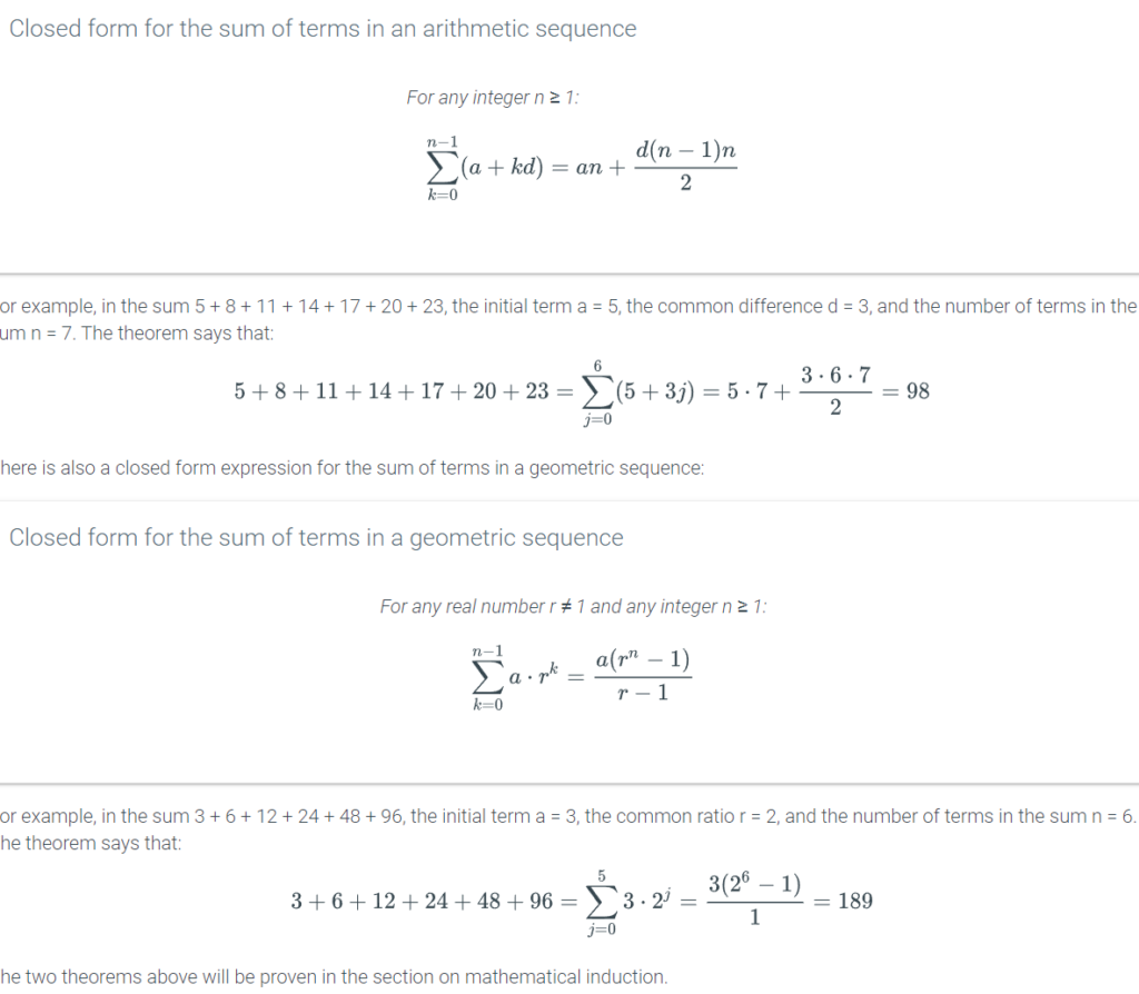
A closed form for a sum is a mathematical expression that expresses the value of the sum without summation notation. There are closed form expressions for some, although not all, of the summations that arise naturally in scientific applications.

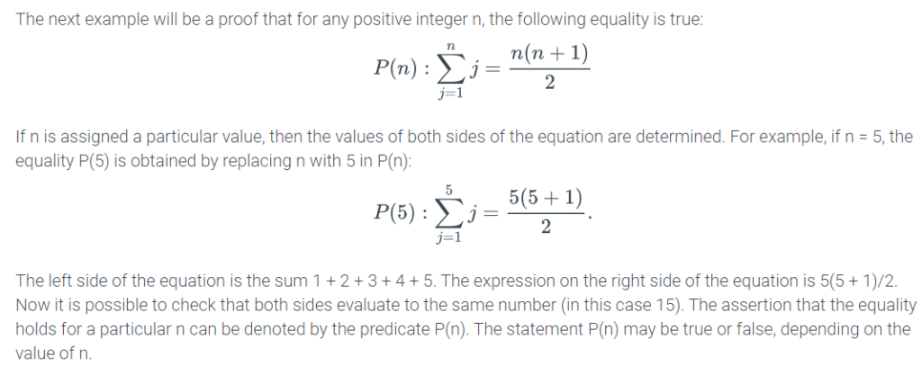
3.8 Lesson: Inductive proof

Lesson introduction

Once the Titanic hit an iceberg and the first bulkhead filled with water, Captain Smith knew the ship would sink. As soon as the first bulkhead filled with the water, he knew the second bulkhead would fill. As soon as the second filled up with water, the third would fill, and like dominos the fourth, fifth,…, and n^th bulkhead would eventually fill. The Titanic had n=16 “watertight” compartments, but as we can see it really did not matter whether n=1 or 1,000,000. Once the first compartment filled, the Titanic was doomed.

We just used induction (not to be confused with inductive reasoning). Knowing that if the n^th compartment filled then the (n+1)^th compartment would fill, is the inductive step.

Induction basics

Suppose that one day a genie grants you three wishes. You make two wishes and then for your third wish, you wish for three more wishes the next day. Given the fact that you can always use your third wish to renew your wishes for the next day, it is possible to prove that from that first day onward, you can have three wishes every day for the rest of your life. This is an example of the principle of mathematical induction (or just induction for short).

The two components of an inductive proof.

• The base case establishes that the theorem is true for the first value in the sequence.
  
  • The genie grants you three wishes on day 1
• The inductive step establishes that if the theorem is true for k, then the theorem also holds for k + 1.
  
  • If you have three wishes on day k, then you can get three wishes for day k+1 (by using the third wish to ask for three more wishes the next day).

The principle of mathematical induction states that if the base case (for n = 1) is true and inductive step is true, then the theorem holds for all positive integers.

Principle of mathematical induction

Let S(n) be a statement parameterized by a positive integer n. Then S(n) is true for all positive integers n, if:

1. S(1) is true (the base case).
2. For all k ∈ Z⁺, S(k) implies S(k+1) (the inductive step).

In the statement “S(k) implies S(k+1)” of the inductive step, the supposition that S(k) is true is called the inductive hypothesis.

Lesson summary

Now that you have completed this lesson you should be able to analyze an inductive proof for validity and flaws. Take a moment to think about what you’ve learned in this lesson:

• The base of an inductive proof is the first case: n=1 or n=0. It is usually proved by simply substituting in 1 or 0 and validating the result.
• The inductive step of an inductive proof is the case that depends on the assumption that the previous steps are true for n and that it is true for n + 1…; or, for all n∈N, f(n) implies f(n+1). Try to think of proofs as a series of if-then statements, e.g., if x is true then it logically follows that y is true.
• To be valid, an inductive proof must have a base case and at least one inductive step.
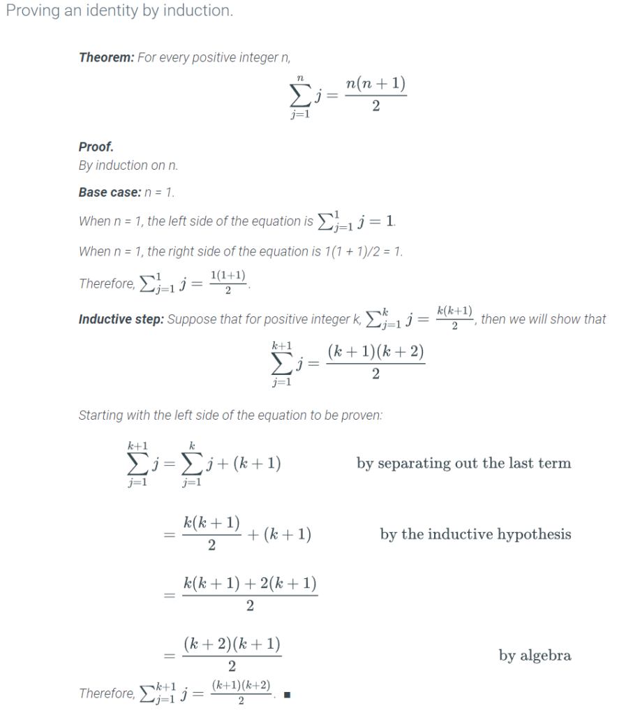
• Use induction to prove that a series is equal to a given formula.
  • Show the base case is true
  • Assume that if it is true for n then it must be true for n + 1.
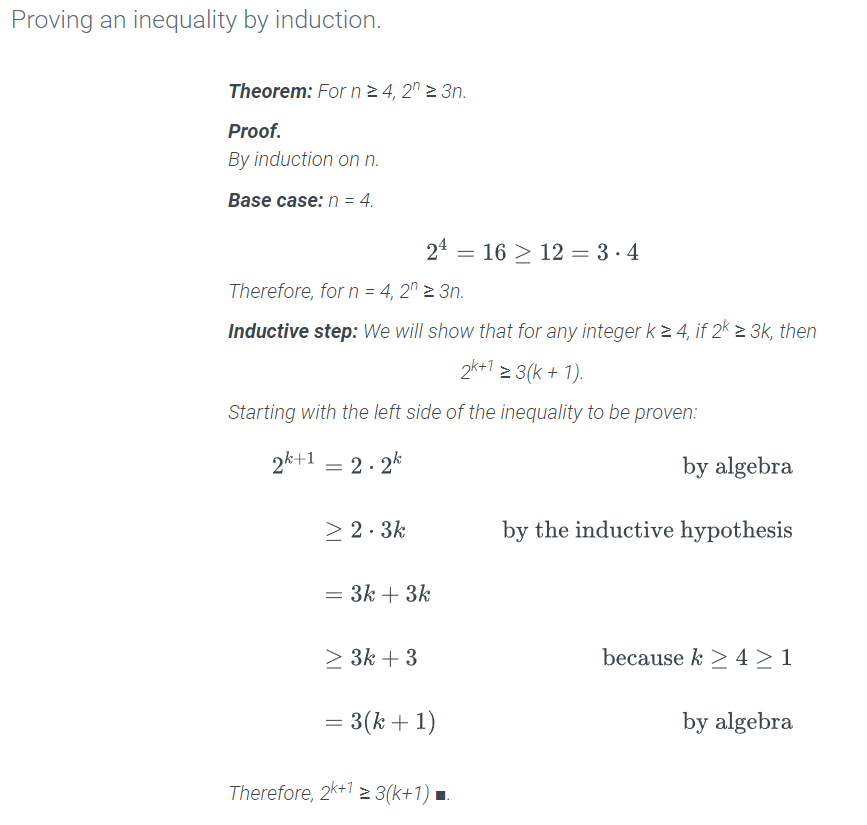
• Use induction to prove that inequalities are true.

3.9 Lesson: Divisibility proof by induction

Lesson introduction

In the previous lesson you learned about the structure and use of an inductive proof. Induction can be used to prove statements about any discrete set that can be ordered (a well-ordered set). That is, any set that can be counted, like your fingers, arranged from least to greatest, and has a smallest value is called a well-ordered set. 

Divisibility proof by induction

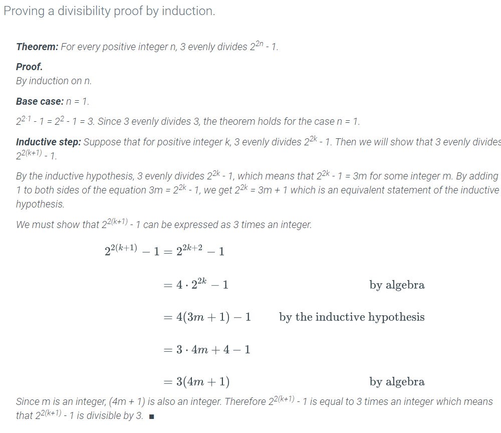
The next example of a proof by induction proves that 3 evenly divides the value of a mathematical expression parameterized by an integer n.

Lesson summary

Now that you have completed this lesson you should be able to analyze a divisibility proof by induction for validity and flaws. Take a moment to think about what you’ve learned in this lesson:

• To determine if a divisibility proof is valid, verify that the given algebraic equation is equivalent to the given statement.
• Identify which statement is equivalent to the inductive hypothesis.
• Write the inductive hypothesis as an equivalent algebraic expression. For example, “for every positive integer n, 2 evenly divides 2ⁿ” as “for some integer m, 2m=2^k“.
• Use induction to prove that a divisibility statement is true.
  • Show it is true for the base case
  • Show that if it is true for n then it must be true for n + 1

3.10 Lesson: Induction proof of a recurrence relation

Lesson introduction

Remember those recurrence relations? Recurrence is connected to many things in computer science, from simple coding to analyzing the runtime of algorithms. When it comes to their computation, you do not want to always rely on brute force. For example, consider the recurrence relation:

This type of formula is called an explicit formula or closed form.

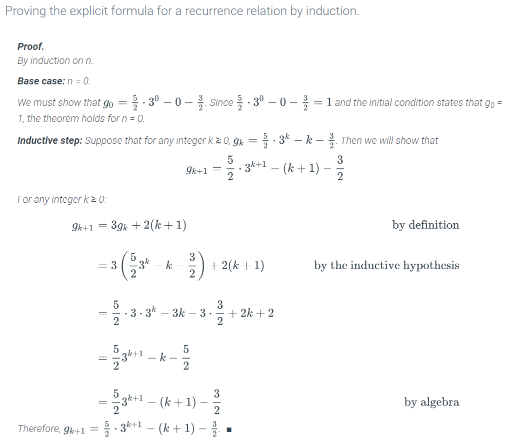
In this lesson you will combine your knowledge of recurrence relations and induction by analyzing an induction proof of a recurrence relation.

Lesson summary

Now that you have completed this lesson you should be able to analyze an induction proof of a recurrence relation for validity and flaws. Take a moment to think about what you’ve learned in this lesson:

• Find the base step of an induction proof by substituting in n = 0 or n = 1.
• Find the inductive step of an induction proof by substituting in n + 1.
• Check that the base and inductive steps of a recurrence proof are satisfied.
• Prove the explicit formula for a recurrence relation using induction. Show the base case by substituting in n = 0 or n = 1. Next substitute n + 1 into the formula. Algebraically manipulate the result so the case for n is separated. The n case is assumed to be true; now leverage this to show that the remaining parts are true. For recursion, this often means isolating the f_n+1 term.

Call with Bob Hoar –

Supplemental Worksheet – doing the proofs is not needed

With a slinky – prove it works –

Take the base case that works and then assume it works for some k

the inductive hypothesis – takes it to the value k – for some values it’s supposed to hold for –

Prove that the theorem holds – for the K + 1

3.11 Lesson: Induction proof of closed summation

Lesson introduction

In the previous lesson, you applied induction to sequences. In this lesson you will continue working with summations (or series). The goal — to find explicit formulas — will be similar, but in this lesson you will find an explicit formula for summations.

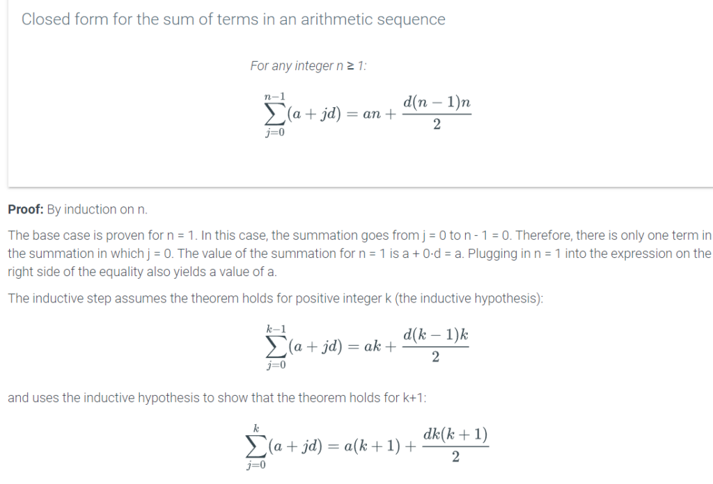
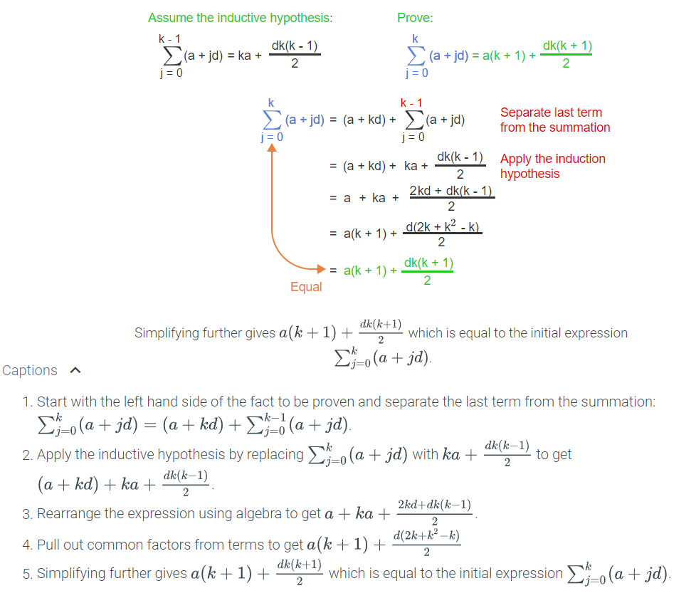
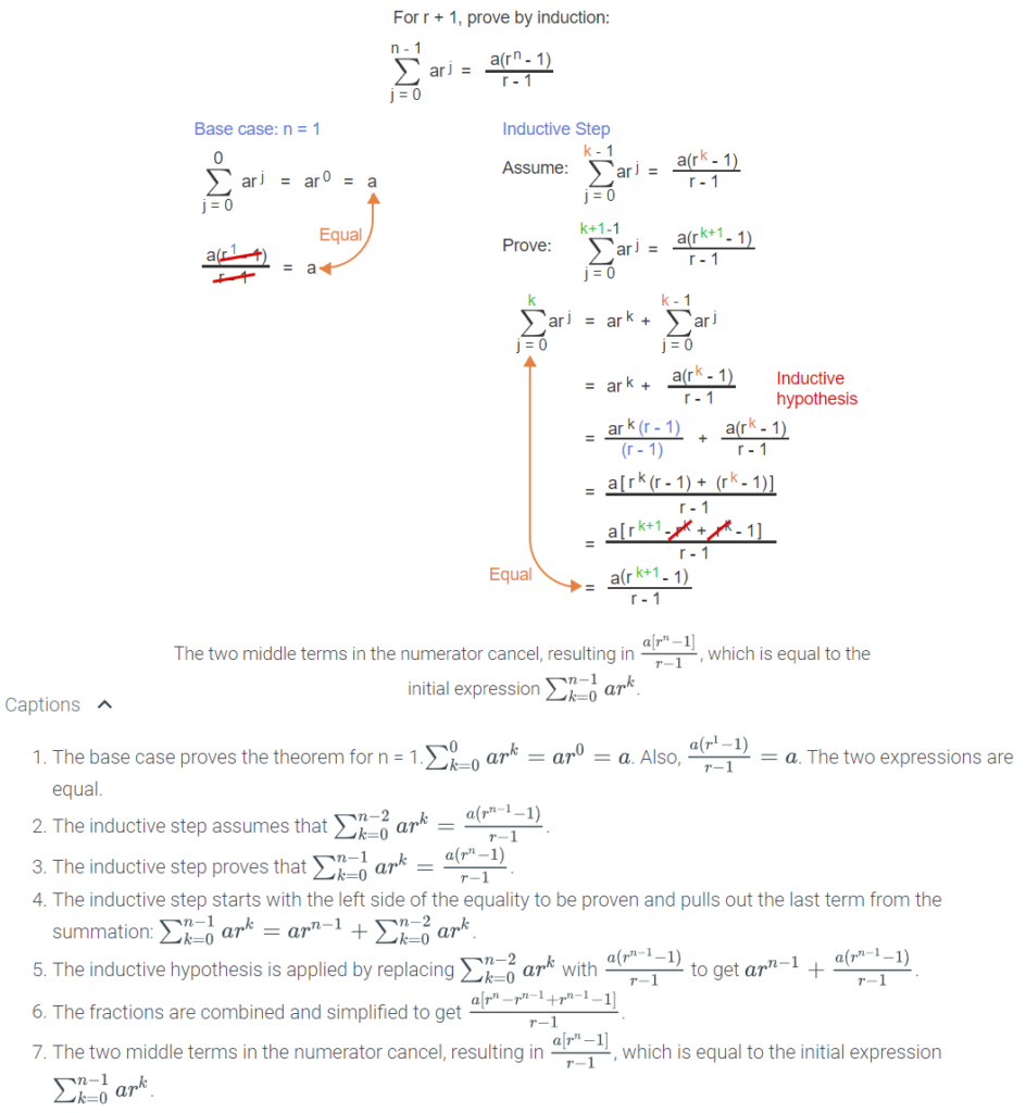
Inductive proofs showing the closed forms for sums of arithmetic and geometric sequences

The theorem below gives a closed form for the sum of the first n terms in an arithmetic sequence. Here we present an inductive proof of the theorem.

Lesson summary

Now that you have completed this lesson you should be able to analyze an induction proof of a closed summation for validity and flaws. Take a moment to think about what you’ve learned in this lesson:

• Find the base step of an induction proof by substituting in n = 0 or n = 1.
• Find the inductive step of an induction proof by substituting in n + 1.
• Check that the base and inductive steps of a summation proof are satisfied.
• Prove the explicit formula for a summation relation using induction. Show the base case by substituting in n = 0 or n = 1. Next substitute n + 1 into formula. Algebraically manipulate the result so the case for n is separated. The n case is assumed to be true; now leverage this to show that the remaining parts are true. With summations, this is often done by separating the last term of the n + 1 case.

3.12 Lesson: Strong induction

Lesson introduction

Induction is like climbing an infinite ladder. You cannot start without taking the first step, the base case. Then you make an induction hypothesis: you assume there is an n^th step. Finally, you show that if an n^th step exists than the (n+1)^th next step, the step, must also exist. This allows the ladder to be climbed. The 1st step exists, so the 2nd must exist, then the 3rd, then the 4th, then the 5th, etc.

The principle of strong induction assumes that the fact to be proven holds for all values less than or equal to k and proves that the fact holds for k+1. By contrast the standard form of induction only assumes that the fact holds for k in proving that it holds for k+1. Define S(n) to be the assertion that f_n ≤ 2ⁿ, where f_n is defined by Fibonacci’s initial values and recurrence relation. The proof that S(n) is true for all non-negative integers n has two components:

• Base case: S(0) and S(1) are true.
• Inductive step: For every k ≥ 1, (S(0) ∧ S(1) ∧ …. ∧ S(k)) implies S(k + 1).

Generalized strong induction: multiple base cases

The predicate S(n) may be true only for n greater than or equal to a particular value denoted below by the constant a. Also, the base case may require proving the assertion directly for more than one value. The base case for a proof by strong induction establishes that S(n) holds for n = a through b, where a and b are constants. The inductive step in a proof by strong induction assumes that S(j) is true for all values of j in the range from a through some integer k ≥ b and then proves that theorem holds for k+1.

Strong induction example: buying cans of juice in 3-packs or 4-packs.

Suppose that cans of juice come in packs of 3 or 4. We would like to be able to buy n cans of juice by purchasing a combination of 3-packs or 4-packs. For which values of n is this possible? Let P(n) be the assertion that it is possible to buy n cans of juice by purchasing only 3-packs or 4-packs. P(7) is true because we can purchase one 3-pack and one 4-pack. P(5) is not true because there is no way to combine 3-packs and 4-packs to get five cans of juice. We will use strong induction to prove that for any n ≥ 6, P(n) is true. Here is an outline of the proof:

• Base case: Prove P(6), P(7), and P(8) directly.
• Inductive step: For k ≥ 8, assume that that P(j) is true for any j in the range 6 through k, and prove that P(k + 1) is true.
  • Argue that P(k – 2) is true by showing that k – 2 falls in the range 6 through k, covered in the inductive hypothesis. The argument uses the fact that k ≥ 8 and therefore k – 2 ≥ 6.
  • Since P(k – 2) is true, k-2 cans of juice can be bought by combining 3-packs and 4-packs. By adding one 3-pack to the k – 2 cans of juice, there will be k – 2 + 3 = k + 1 cans of juice. Therefore P(k + 1) is true

Lesson summary

Now that you have completed this lesson you should be able to analyze proofs using strong induction and generalized strong induction for validity and flaws. Take a moment to think about what you’ve learned in this lesson:

• The notation used in inductive steps in strong and generalized induction is: for every k≥1,S(0)∧S(1)∧S(2)∧…∧S(k); it means for case from the base of to the k^th case.
• When using strong induction, you must assume that the statement is true for n and assume that all the previous cases are also true. That is, you must show that it is true for S(0) and then assume that S(0) through S(k) are true.
• When using generalized induction, you must show the base cases up to the i^th case are true and then assume that every case afterwards is true. For example, show that S(0), S(1) and S(3) are true and then assume that S(3) through S(k) are true.

3.13 Lesson: Well-ordering principle

Lesson introduction

Consider the statement: any postage costing ≥8 cents must be paid with 5 and 3 cent stamps. How could you prove this?

Since you are assuming it exists (though it actually does not) then by the well-ordering principle there is a smallest number for which you cannot make postage; let’s call this number n. You can pay 8 = 3(1) + 5(1), and 9 = 3(3) + 0(5), and 10 = 3(0) + 5(2) postage; so n≥11. Now here is the trick. Using the well-ordering principle, you know that n is the smallest postage you could not pay.

The well-ordering principle says that any non-empty subset of the non-negative integers has a smallest element.

Let P(n) be a predicate that is parameterized by non-negative integers n. If the following two conditions hold:

• Base case: S(1) is true
• Inductive step: For all k ≥ 1, S(k) implies S(k+1)

then for all n ≥ 1, S(n) is true.

Proof that well-ordering implies the principle of mathematical induction.

Proof.

Proof by contrapositive: We will show that if the well-ordering principle is true and S(n) is false for some n ≥ 1, then at least one of the two conditions for induction must fail.

Suppose that S(n) is false for some n ≥ 1. Consider the set of integers n such that n ≥ 1 and S(n) is not true. By the well-ordering principle, there must be a smallest element m in that set. Note that m ≠ 0 because 0 is not a member of the set. (One of the criteria for an integer n to be included in the set is that n ≥ 1.) If m = 1, then S(1) is not true and the base case fails. If m ≥ 2, then S(m – 1) is true but S(m) is false. Letting k = m – 1, k ≥ 1 and S(k) is true but S(k + 1) is not true. Therefore, the inductive step fails for some k ≥ 1. Thus, if the statement S(n) is false for some n ≥ 1, then one of the two conditions for the principle of mathematical induction must be false.  ■

roof of the quotient and remainder theorem using the well-ordering principle

Proof.

Consider the set S of all non-negative integers of the form (n – td), where t is an integer. The set is non-empty because t can be chosen so that -td is as large as desired and large enough to make (n – td) non-negative. Let r be the smallest number in the set S and let q be the value for t which achieves the minimum: r = n – qd. By definition, r is non-negative and therefore r ≥ 0. The fact that r < d will be proven by contradiction. Suppose that r ≥ d. Then r – d ≥ 0.

Since r – d can be written in the form (n – td) by selecting t = q + 1, r was not the smallest non-negative number in the set of integers of the form n – td. A contradiction.  ■

Lesson summary

Now that you have completed this lesson you should be able to analyze proofs using the well‐ordering principle for validity and flaws. Take a moment to think about what you’ve learned in this lesson:

• Use the following three steps to apply the well-ordering principle:
  • Define a set of counterexamples
  • Assume the set is not empty; by the well-ordering principle, a minimum element exists
  • Use the existence of the minimum element to reach a contradiction

3.14 Module 11: Recursive Structures

This page marks the beginning of Module 11. This module contains four lessons:

• Overview of recursive definitions
• Recursively defined sets
• Recursion for perfect binary trees
• Recursive/inductive algorithms

3.15 Lesson: Overview of recursive definitions

Lesson introduction

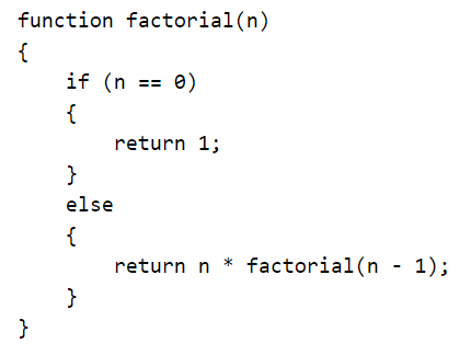
In Unit 1 you learned about the various types of algorithms, some of which use iterations to compute an output. Iteration and recursion are key concepts used in computer science. The factorial example below might be coded as follows:

Lesson summary

Now that you have completed this lesson you should be able to apply recursive rules to obtain an output from a recursive definition for a function. Take a moment to think about what you’ve learned in this lesson:

• The basis of a recursive definition is the initial term(s), usually denoted �(0).
• Similar to a recurrence relation, the recursive rule in a function defines how to find the next term using previous terms. It is denoted �(�) and should be read as the value output for the n^th time the recursion rule has been applied. Tip: Do not confuse this with function notation that you may recall from calculus, e.g., �(�)=3�2+1⇒�(2)=3(2)2+1=13.
• To compute the n^th value of function defined recursively:
  • apply the recursive rule to the basis value,
  • apply the rule to the output, and
  • repeat as many times as necessary.

3.16 Lesson: Recursively defined sets

Lesson introduction

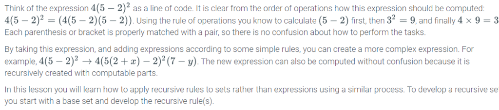
Recursively defined sets

Certain kinds of sets are most naturally specified with recursive definitions. A recursive definition of a set shows how to construct elements in the set by putting together smaller elements.

Components of a recursive definition of a set

• A basis explicitly states that one or more specific elements are in the set.
• A recursive rule shows how to construct larger elements in the set from elements already known to be in the set. (There is often more than one recursive rule).
• An exclusion statement states that an element is in the set only if it is given in the basis or can be constructed by applying the recursive rules repeatedly to elements given in the basis.

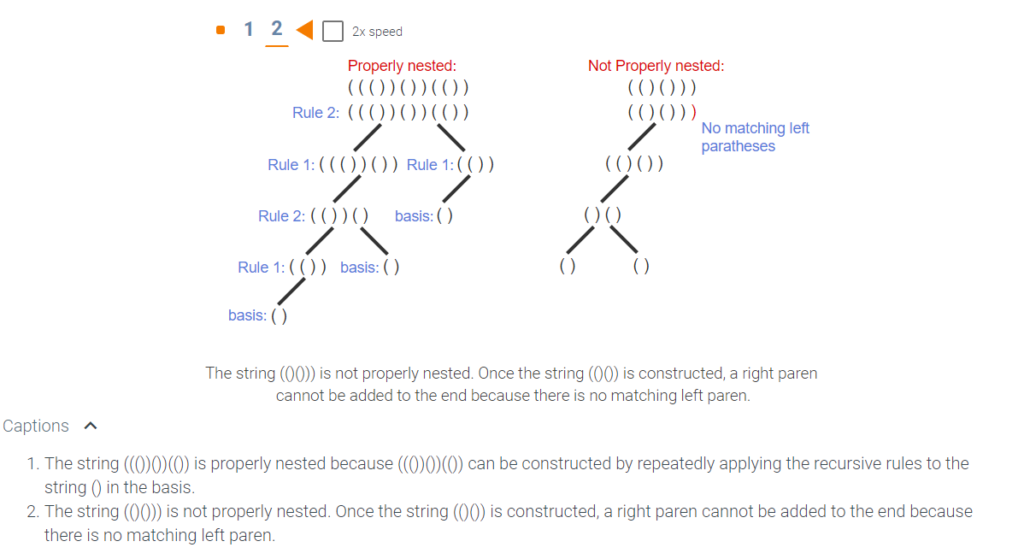
Recursive definition of the set of all properly nested parentheses.

• Basis: The sequence () is properly nested.
• Recursive rules: If u and v are properly-nested sequences of parentheses then:
  
  1. (u) is properly nested.
  2. uv is properly nested.
• Exclusion statement: a string is properly nested only if it is given in the basis or can be constructed by applying the recursive rules to strings in the basis.

Lesson summary

Now that you have completed this lesson you should be able to apply recursive rules to obtain an output from a recursive definition for a set. Take a moment to think about what you’ve learned in this lesson:

Recursive definition of the set of all properly nested parentheses.

• Basis: The sequence () is properly nested.
• Recursive rules: If u and v are properly-nested sequences of parentheses then:
  
  1. (u) is properly nested.
  2. uv is properly nested.
• Exclusion statement: a string is properly nested only if it is given in the basis or can be constructed by applying the recursive rules to strings in the basis.

• A recursive definition of a set shows how to construct elements in the set by putting together smaller elements.
• Components of a recursive definition of a set include:
  • A basis that explicitly states one or more specific elements are in the set.
  • Recursive rules that shows how to construct larger elements in the set from elements already known to be in the set.
  • An exclusion statement that states that an element is in the set only if it is given in the basis or can be constructed by applying the recursive rules repeatedly to elements given in the basis.

3.17 Lesson: Recursive definition for perfect binary trees

Lesson introduction

In Discrete Mathematics I you learned about binary relations and how to represent the relations as trees. In this lesson you will apply your knowledge of recursive definitions to construct perfect binary trees. If you forgot about trees don’t worry, the beginning of the lesson provides a review of the terminology and structure of binary trees.

Recursive definition for perfect binary trees

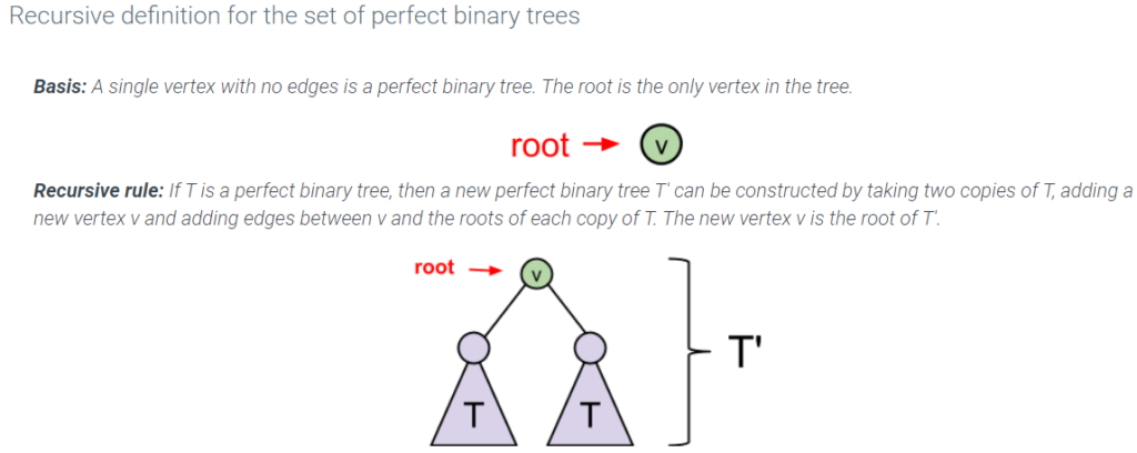
The next example is a recursive definition for a set of mathematical objects that are not strings. A tree has vertices (denoted by a circle) and edges (denoted by line segments) which connect pairs of vertices. Not every collection of vertices and edges is a tree. A formal definition of trees along with their properties is given elsewhere in this material. Here we give a recursive definition for a particular class of trees called perfect binary trees. Each perfect binary tree has a designated vertex called the root.

Lesson summary

Now that you have completed this lesson you should be able to apply recursive rules to construct a perfect binary tree given a recursive definition for a binary tree. Take a moment to think about what you’ve learned in this lesson:

• The number of steps necessary to construct a perfect binary tree can be determined by counting the height in number of vertices below the root (the root does not count).
• To construct a perfect binary tree, draw the root (a single vertex), and then draw two lines each ending with a vertex. From each of these new vertices, draw two more lines with vertices. Repeat as many times as necessary. Because you are doubling the number of vertices each time, the n^th step should have 2ⁿ vertices.

3.18 Lesson: Recursive/inductive algorithms

Lesson introduction

Now that you know how to apply recursive rules to functions, sets, and trees, it is time to apply it to algorithms using pseudocode. Fortunately, you will be given the blueprint. To execute a recursion in an algorithm is similar to the other structures. You will need a starting point for the code and a well-defined method to derive the next step from previous information.

Recursive algorithm

A recursive algorithm is an algorithm that calls itself. Like recursively defined sequences and structures, a recursively defined algorithm has a base case in which the output is computed directly on an input of small size or value. On a larger input, the algorithm calls itself on an input of smaller size and uses the result to construct a solution to the larger input. An algorithm’s calls to itself are known as recursive calls. Here is an example of a recursive algorithm to compute n!. Comments in the pseudo-code, which begin with “//”, explain the purpose of certain steps and are not part of the algorithm itself.

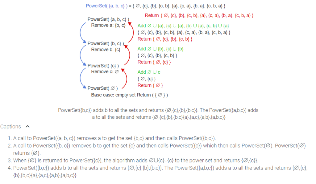
Recursive algorithm to compute the power set of a set

PowerSet(A)

Input: A set A.
Output: The power set of A.

If (A = ∅)
    Return( {∅} )

Select an element a ∈ A
A’ := A – {a}
P := PowerSet(A’)  //the recursive call
P’ := P
For each S ∈ P’
    Add S∪{a} to P
End-for

Return( P )

Lesson summary

Now that you have completed this lesson you should be able to determine a corresponding output value for a given input and recursive algorithm written in pseudocode. Take a moment to think about what you’ve learned in this lesson:

• The base case in an algorithm is the same concept as the basis of a recursive definition. It is the return value for n=0.
• The recursive call is the same as the recursive rule of a definition. It is the return value for input greater than the basis (n≥1).
• To determine the output for pseudocode, find the recursive call value for the basis. Then find the recursive call value of that value and repeat as many times as instructed. Hint: The process is identical to finding values using recursive rules or sequences.

3.19 Module 12: Simple Recurrence Relations

This page marks the beginning of Module 12. This module contains two lessons:

• Introduction to linear homogeneous recurrence relations
• Solving linear homogeneous recurrence relations problems

3.20 Lesson: Linear homogeneous recurrence relations

Lesson introduction

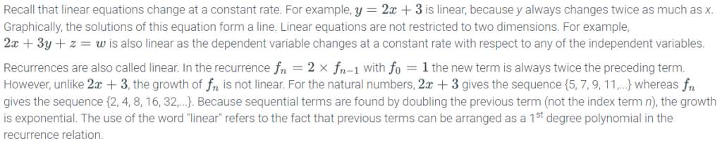
Recall that linear equations change at a constant rate.

Linear homogeneous relations

There are many different kinds of recurrence relations, some of which are very difficult to solve. There are also recurrence relations for which there are no known explicit formula. This material focuses on a particular class of recurrence relations called linear homogeneous recurrence relations. Each number in a sequence defined by a linear homogeneous recurrence relation is a linear combination of numbers that occur earlier in the sequence.

Lesson summary

Now that you have completed this lesson you should be able to identify linear homogeneous recurrence relations. Take a moment to think about what you’ve learned in this lesson:

3.21 Lesson: Solving a recurrence relations problem

Lesson introduction

Solving a linear recurrence relation

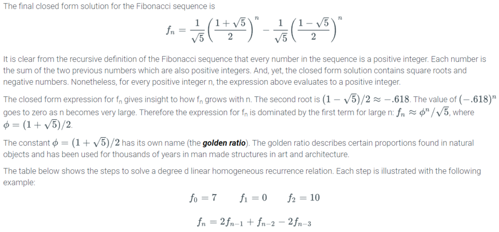
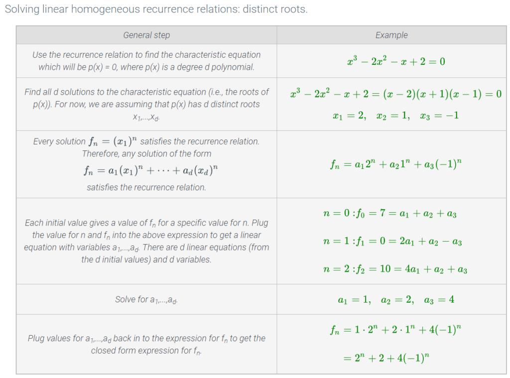
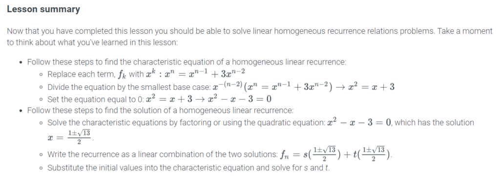
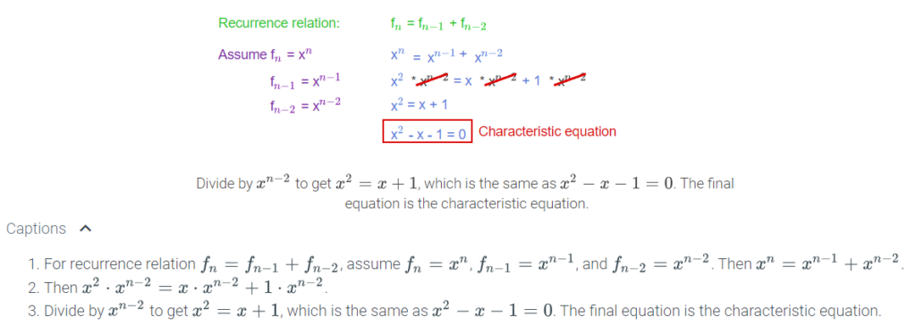
To solve a linear recurrence relation, we start with the guess that f_n has the form xⁿ for some x. While there are mathematical tools to derive the solution to linear homogeneous recurrence relations without resorting to a guess, we know from experience that an exponential function is a good place to start. Plugging in the exponential expression into the recurrence relation, gives rise to an equation called characteristic equation for the recurrence. The characteristic equation for a linear recurrence relation can be used to solve for x, the base of the exponent in the solution. The following animation illustrates for the Fibonacci recurrence relation:

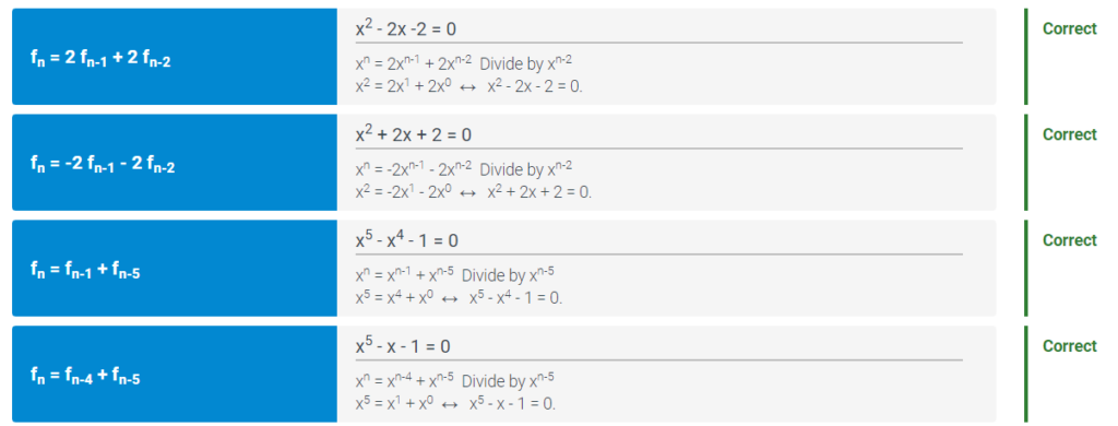
Once the characteristic equation has been determined, the next step is to find all values of x that solve the equation. Since the characteristic equation has the form p(x) = 0, for some polynomial p(x), the goal is to find the roots of the polynomial. Some polynomials have complex roots. This material only covers the case where the characteristic equation has real roots. We first consider the case where all the roots are distinct. For example, the characteristic equation for the Fibonacci sequence gives rise to the binomial equation:

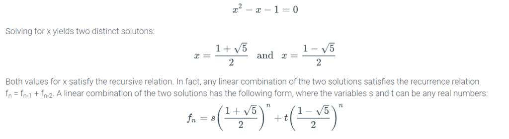
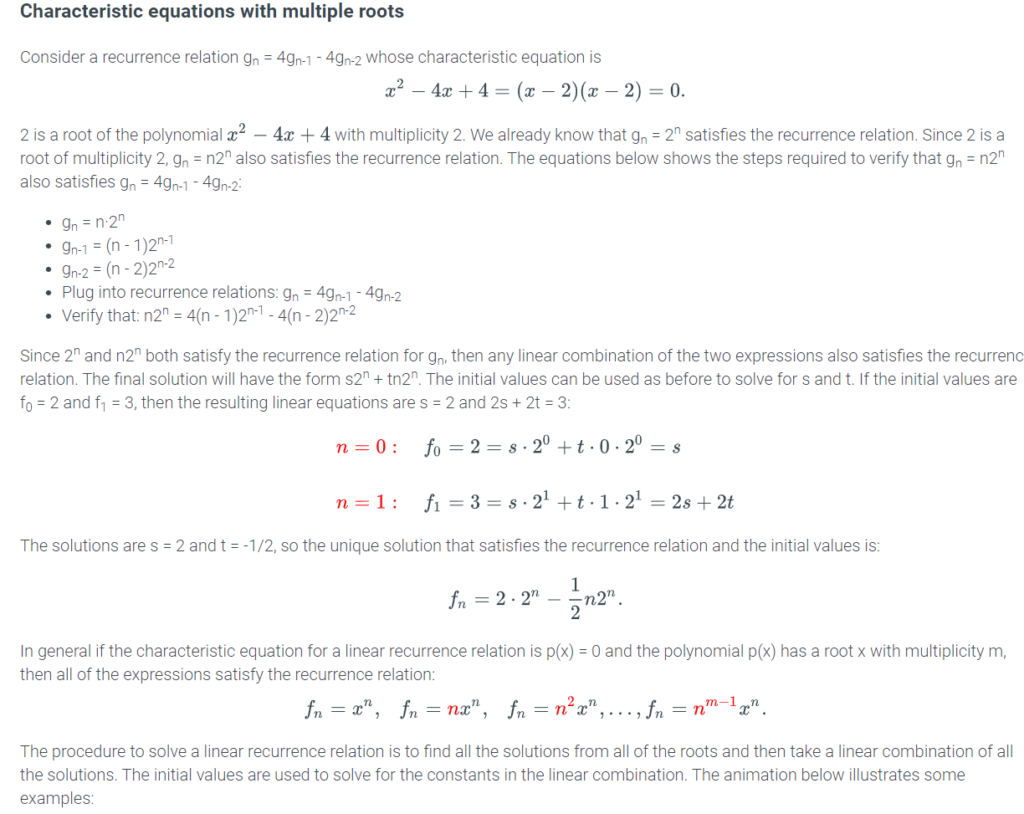
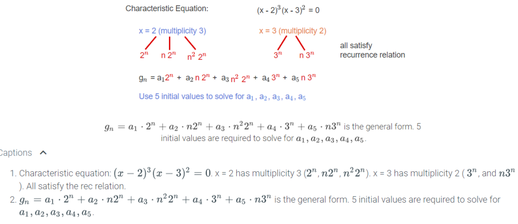
Thus, there are an infinite number of solutions to the recurrence relation. However, not all of the solutions satisfy the initial values. The expression denoting the infinite set of solutions to a recurrence relation without initial values is called the general solution to the recurrence relation. The initial values add constraints that narrow down the set of possible solutions to particular values for s and t. To summarize, if x and y are solutions to the characteristic equations, then f_n = xⁿ and f_n = yⁿ both satisfy the recurrence relation. Furthermore any linear combination of xⁿ and yⁿ satisfy the recurrence relation as is stated more formally in the theorem below: