1.1 Unit 1: Algorithms

This is the beginning of Unit 1 in this Discrete Mathematics II course.

The material in this unit comprises 13% of the high-stakes assessment and includes such concepts as:

• Algorithms
• Evaluating algorithm complexity
• Worse case analysis
• Asymptotic growth
• Algorithms and big-o notation

1.2 Module 1: Algorithm Structures

This page marks the beginning of Module 1. This module contains five lessons:

• Introduction to algorithms
• If-then algorithms
• For-loop algorithms
• While-loop algorithms
• Nested loop algorithms

1.3 Lesson: Introduction to algorithms

Lesson introduction

The module introduction introduced the concept of an algorithm, which tells the computer exactly what to do in a precise, step-by-step fashion. No matter which programming language is used, there are three basic building blocks of an algorithm: assignments, conditional statements, and loops. Pseudocode uses specifically formatted natural-language- like statements to capture these steps in the algorithm.

An important type of step in an algorithm is an assignment, in which a variable is given a value. An assignment operator is denoted by:

x := y

The output of an algorithm is specified by a return statement. 

 

Lesson summary

Now that you have completed this lesson you should be able to interpret pseudocode for an algorithm. Take a moment to think about what you’ve learned in this lesson:

• An algorithm is a step-by-step method for solving a problem. A description of an algorithm specifies its input, output, and the sequence of steps to obtain the output from the input. A description of an algorithm usually includes the name of the algorithm, a brief description of the task performed by the algorithm, a description of the input, a description of the output, and the sequence of steps to follow.
• Algorithms are often described using pseudocode, which is a detailed yet readable description of what an algorithm must do.
• An assignment statement in pseudocode gives a value or changes the value of a variable. In pseudocode assignment statements that give the value of an expression to a variable are written as variable := expression.
• The return statement returns values as output from an algorithm when used at the end of an algorithm. When used in the middle of an algorithm, it stops its execution and provides the most recent value of a variable or an expression. In pseudocode the return statements are written as Return(expression), where the expression defines the evaluated value.

1.4 Lesson: If-then algorithms

Lesson introduction

In the previous lesson you were introduced to the terminology and structure of an algorithm that presents a series of steps. In this lesson you will learn two of the most basic types of algorithms: if-then and if-then- else algorithms.

If-statements

An if-statement tests a condition, and executes one or more instructions if the condition evaluates to true. 

If-else statements

An if-else-statement tests a condition, executes one or more instructions if the condition evaluates to true, and executes a different set of instructions if the condition evaluates to false. 

Lesson summary

Now that you have completed this lesson you should be able to determine the corresponding output value when given an input value and pseudocode for an if‐then or if‐then‐else algorithm. Take a moment to think about what you’ve learned in this lesson:

• An if-then statement tests a condition and executes one or more steps if the condition is true. An if-else statement tests the condition, and executes one or more instructions if the condition is true, and another instruction or set of instructions if it is false.
• The structure of the if-then statement in pseudocode when there is only one step to execute when the condition is true is:
  If(condition), step
• When multiple steps should be performed upon a true condition, the steps are indented and the end of the list of steps is noted with an End-if statement:  If (condition) Step 1 Step 2 ... Step n End-if
• The if-else statement in pseudocode is formatted in the following format:  If (condition) One or more steps Else One or more steps End-if
• When needed, if-then and if-else statements can be nested. There are no limitations regarding how many if-then or if-else statements can be placed under another if-then or if-else statement. You will learn more about nested statements later in this module.

1.5 Lesson: For-loop algorithm

Lesson introduction

Algorithms frequently require steps to be executed several times. Programming languages provide various iterative mechanisms to determine the start and end points in a loop. They are a quick and easy way to do something repeatedly. Together with assignment and conditional statements, looping statements (iterations) are the basic building blocks of algorithms. An iteration is a process where a set of instructions or structures are repeated in a sequence a specified number of times or until a condition is met.

To control the iterations, for-loops use an index or a counter and a variable that counts how many times a step or a block of steps executes. The index and counter variable specify the initial value of the counter and a step, or block of steps, to be executed before the counter is increased by 1. The statement or statements in the block will be executed for the incremented value of the counter over and over until the counter reaches its maximum specified value.

Lesson summary

Now that you have completed this lesson you should be able to determine the final output and values during iterations of a for‐loop algorithm written in pseudocode. Take a moment to think about what you’ve learned in this lesson:

• Looping structures provide a means of specifying a sequence of steps that are to be repeated. For-loops are used when the number of iterations in the loop is known.
  • They are controlled by an index that is specified a starting and a final value.
  • The first iteration of the loop executes for the initial value of the index, which increments by 1 for every iteration, until it reaches its final value.
  • For-loops perform at least one iteration for the initially assigned value of the counter.
• For-loops use the following syntax in pseudocode:  For index=start_value to final_value One or more steps End-for
• The for-loop iterates final_value-start_value+1 times.

1.6 Lesson: While-loop algorithm

Lesson introduction

When looping is needed some algorithms cannot specify the number of iterations but rely on evaluating a condition to determine if there will be an additional iteration. While-loop algorithms are used when the decision if another iteration is needed or not is based on evaluating a condition. While-loops iterate as long as the specified condition is true. They repeat a specific block of code an unknown number of times until the condition is met. A while-loop iterates an unknown number of times, ending when a certain condition becomes false. A while-loop is written as follows:

While ( condition )
    Step 1
    Step 2
    . . .
    Step n
End-while

Lesson summary

Now that you have completed this lesson you should be able to determine final output and values during iterations of a while-loop algorithm written in pseudocode. Take a moment to think about what you’ve learned in this lesson:

• While-loops are used when the number of iterations in the loop is unknown and may execute zero or more iterations. They are controlled by a conditional statement. If the conditional statement is true, the loop initiates an iteration otherwise it stops.
• While-loops use the following syntax in pseudocode:  While (condition) One or more steps End-while
• The while-loop iterates zero or more times until the condition is met.

1.7 Lesson: Nested loop algorithm

Lesson introduction

Assignment, conditional, and iterative statements could comprise steps that execute in an iteration. Placing a loop within another loop is known as nesting. When a loop exists within another loop, it is called a nested loop. Both for- and while- loops can be nested in other for- or while-loops

Nested loops

A nested loop is a loop that appears within another loop. The nested loop, known as the inner loop, is treated as a sequence of steps inside the outer loop. A nested loop is illustrated below in an algorithm that counts the number of duplicate pairs in a sequence of numbers.

Lesson summary

Now that you have completed this lesson you should be able to determine the final output and values during iterations of a nested loop algorithm written in pseudocode. Take a moment to think about what you’ve learned in this lesson:

• Loops can be nested.
• The outer loop controls the execution of the inner loop.
• While-loops can nest in for-loops, and vice-versa; loops of the same type can also nest.
• The outer loop takes control of the number of complete repetitions of the inner loop.
  • The first pass of the outer loop triggers the inner loop, which executes to completion.
  • Then the second pass of the outer loop triggers the inner loop again.
  • This repeats until the outer loop finishes.

1.8 Module 2: Analyzing Algorithms

This page marks the beginning of Module 2. This module contains three lessons:

• Computational complexity
• Evaluating algorithm complexity
• Worst-case analysis

1.9 Lesson: Computational complexity

Lesson introduction

In the previous module you learned that algorithms have three basic building blocks: assignments, branches, and loops. When you write an algorithm, you combine the building blocks to define the steps that need to be completed in order for the algorithm to achieve its goal, providing a solution to a problem.

In this lesson you will learn about algorithm complexity, which is the study of the efficacy of algorithms that gives us a framework to compare algorithms.

Computational complexity

An algorithm describes the underlying method for how a computational problem is solved. The primary resources to optimize are time complexity, the time the algorithm requires to run, and space complexity, the amount of memory used. Together they are respectively referred to as time and space complexity of the algorithm.

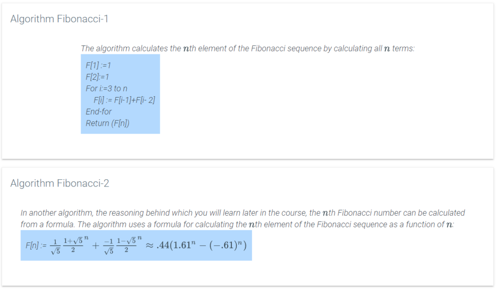
The algorithm Fibonacci-2 only needs the value of n to be plugged in, and then there are a few additions, subtractions (equivalent to additions of negated numbers), multiplications, exponentiations (which are repeated multiplications), and division operations. Regardless of how large n is, the same number of arithmetic operations will be completed.

When n is large, the algorithm Fibonacci-1 will need more and more calculations, while the Fibonacci-2 will not. Both algorithms will give the same output for a given n.

Lesson summary

Now that you have completed this lesson you should be able to describe the computational complexity problems of algorithms. Take a moment to think about what you’ve learned in this lesson:

• The choice of algorithms can heavily influence the efficiency of a solution to a computing problem.
• Computational complexity is a measure of the resources an algorithm uses.
• Time complexity measures the time an algorithm needs to complete.
• Space complexity measures the amount of memory an algorithm uses during its execution.

1.10 Lesson: Evaluating algorithm complexity

Lesson introduction

As you learned in the previous lesson, algorithms need time and space to execute. 

Algorithms and time complexity

As you may recall from the previous module, each algorithm uses assignments, conditional statements, and loops, and performs a variety of operations, such as addition and multiplication. These operations (e.g., addition, multiplication, comparison) that one would find in a single line of pseudocode, are referred to as atomic operations

Lesson summary

Now that you have completed this lesson, you should be able to count the number of atomic operations in a given algorithm. Take a moment to think about what you’ve learned in this lesson:

• A computer problem might have many different algorithms to describe solutions. To optimize computer resources, computer scientists select those that complete in reasonable time.
• Atomic operations are the building blocks of the pseudocode and are considered in assessing the complexity of an algorithm. Atomic operations cannot be split any further; a computer would evaluate each in one step.
• The following are examples of atomic operations:
  • Assigning a value to a variable
  • Looking up the value of a particular element in a sequence
  • Comparing two values
  • Arithmetic operations such as addition and multiplication, including incrementing a value.
• Size of an input is the variable that is used to express the function describing how much time an algorithm needs to complete. It is usually the number of elements in an input sequence.
• Use these guidelines to count the number of atomic operations:
  • Count each assignment as one operation
  • Multiply the operations in the body of the loop by the number of iterations of the loop
  • Ignore constant factors; focus on the elements of the functions that grow the fastest
• Specific features of computing systems, such as processor speed, are not considered when comparing how the time to complete an algorithm grows as the size of the input grows.

1.11 Lesson: Worst-case analysis

Lesson introduction

As algorithms branch and loop depending on various conditions, it is difficult to calculate the number of atomic operations some algorithms perform for all inputs of a given size.

Lesson summary

Now that you have completed this lesson you should be able to analyze the worst‐case time complexity of an algorithm. Take a moment to think about what you’ve learned in this lesson:

• Algorithms are compared by their average running and best running times.
• Worst-case complexity is used to estimate how much time might be needed in the worst case to guarantee that the algorithm will always finish on time.
• Average performance and worst-case performance are the most used in algorithm analysis.

1.12 Module 3: Big-O Estimates

This page marks the beginning of Module 3. This module contains two lessons:

• Asymptotic growth
• Algorithms and big-O

MODULE OBJECTIVE: By the end of this module, you should be able to analyze algorithms for complexity and runtime using big‐O notation.

1.13 Lesson: Asymptotic growth

Lesson introduction

In the previous module you learned about analyzing the worst-case running time of an algorithm by analyzing its pseudocode. In this lesson you will learn about asymptotic complexity—the behavior of the complexity function as n grows. 

Asymptotic behavior

Given the size of an input and a function that counts the number of operations of an algorithm, you can have a pretty good idea of how fast an algorithm is. But the process of counting instructions in your algorithms every time you look at or write an algorithm can become tedious and time consuming. There is a better way to perform complexity analysis, and that is by using big-O notation.

Example: Linear search

The following pseudocode describes an algorithm that checks if the value V exists in the array a[1], a[2],…,a[n]:

For i: = 1 to n If a[i]: = V, return (true) End-for Return(false)

This method of searching for a value within an array is called linear search. The asymptotic complexity for this algorithm is n due to the single for-loop. 

Rule of thumb

• Simple programs can be analyzed by counting the nested loops of the program.
  • A single loop over n items yields asymptotic complexity n.
• If you have a program that calls a function within a loop and you know the number of atomic operations the called function performs, it is easy to determine the number of atomic operations of the whole program. For example, let’s consider the following algorithm:
  For i: = 1 to n f(n) End-forSince you know that f(n) is a function that performs exactly n instructions, you then know that the number of instructions of the whole program is asymptotically n², as the function is called exactly n times.
• Given a series of for-loops that are sequential, the slowest of them determines the asymptotic behavior of the program.
• Two nested loops followed by a single loop is asymptotically the same as the nested loops alone, because the nested loops dominate the simple loop.

Asymptotic notation

Asymptotic notation is a basic mathematical tool for working with functions that we only know up to a constant factor. There are three types of asymptotic notation that are commonly used in algorithmic analysis, O(n) (“big-O”), Ω(n) (“Omega”), and Θ(n) (“Theta”).

• The big-O notation—O(n)—serves as a rough upper bound for functions (disregarding constants and small input values).
• The Ω notation—Ω(n)—is similar to big-O, except that it provides a lower bound on the growth of a function.
• The Θ notation—Θ(n)—indicates how the algorithm performs for any case. This is referred to as an average time or random case function and, when possible, gives us a sense of how the algorithm performs in any case. Note that it is often possible to estimate upper and lower bounds, but not average cases especially if there are complex branching in the code.

Lesson summary

Now that you have completed this lesson you should be able to describe asymptotic growth and the use of omega, theta and big‐O notation. Take a moment to think about what you’ve learned in this lesson:

• Asymptotic complexity describes the behavior of the complexity function as n grows. Only the terms that grow fastest in a complexity function significantly influences its asymptotic complexity, so they are retained without constant multipliers.
• To find the asymptotic behavior for the given function, drop the constant factors and keep the terms that grow the fastest. For example, in this function: 6n + 4, drop the 4 because it remains constant and the constant multiplier 6.
• An algorithm without loops has a constant asymptotic complexity of 1, since the number of instructions it needs is just a constant.
• Any program with a single loop which goes from 1 to n will have asymptotic complexity n, since it will do a constant number of instructions before the loop, a constant number of instructions after the loop, and a constant number of instructions within the loop which all run n times.
• If you cannot readily decide which one of the terms grows faster, plug in several large values for n and compare.
• A single loop that iterates up to n times has a linear asymptotic complexity.
• The asymptotic complexity of a loop nested in a loop is quadratic.

1.14 Lesson: Algorithms and big-O

Lesson introduction

In many cases it is challenging to describe the asymptotic complexity of an algorithm. For comparison purposes and for planning for resources, it often suffices to know that an algorithm will always need more or less resources than described by a function that bound it from above or below.

Big-O and Big-Omega notations

As you may recall from the previous lesson, asymptotic notation is a basic mathematical tool for working with functions that we only know up to a constant factor. There are three types of asymptotic notation that are commonly used in algorithmic analysis: O(n) (“big-O”), Ω(n) (“Omega”), and Θ(n) (“Theta”).

Lesson summary

Now that you have completed this lesson you should be able to analyze the complexity of algorithms whose runtime varies with a given input using big‐O notation. Take a moment to think about what you’ve learned in this lesson:

• Big-O, Omega, and Theta are formal notational methods for stating the growth of resource needs (time and storage) of an algorithm.
• The function that counts the atomic operations of an algorithm falls under the big-O function.
• The function that counts the atomic operations of an algorithm is above the Omega function.
• The Theta function falls between the big-O and Omega functions.