1.1 Relational model

Database models

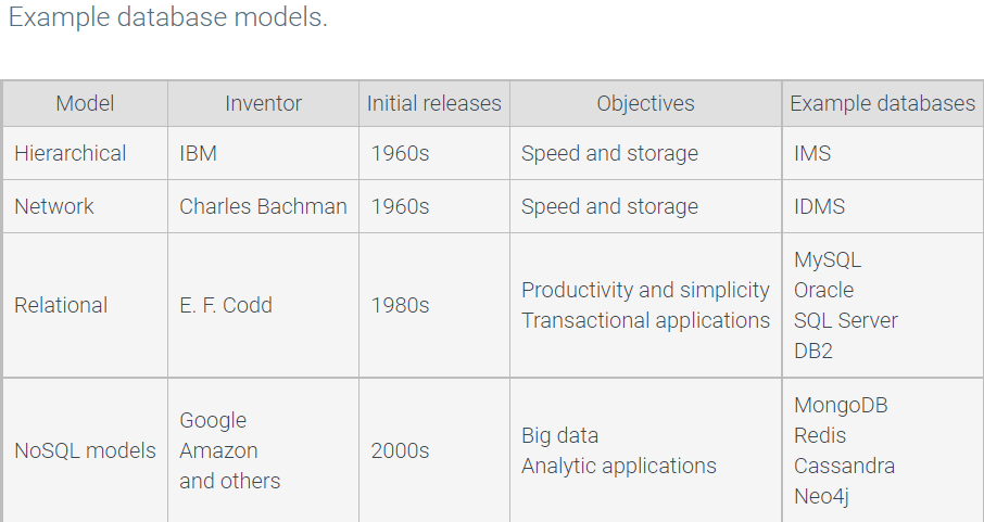
A database model is a conceptual framework for database software.

NoSQL databases. NoSQL stands for ‘Not only SQL’ and encompasses a variety of database models. 

Relational data structure

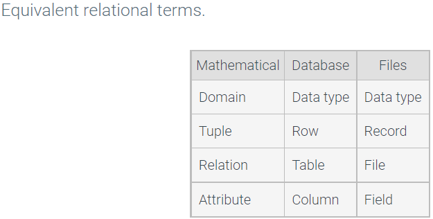
The relational model is a database model based on mathematical principles, with three parts:

1. A data structure that prescribes how data is organized.
2. Operations that manipulate data structures.
3. Rules that govern valid relational data.

A set is a collection of values, or elements, with no inherent order.

Each tuple position is called an attribute.

Relational operations

The relational model stipulates a set of operations on tables, collectively called relational algebra.

Relational operations include:

• Select — selects a subset of rows of a table.
• Project — eliminates one or more columns of a table.
• Product — lists all possible combinations of rows of two tables.
• Join — a product operation followed by a select operation.
• Union — combines two tables by selecting all rows of both tables.
• Intersect — combines two tables by selecting only rows common to both tables.
• Difference — combines two tables by selecting rows that appear in one table but not the other.

Relational rules

Relational rules, also known as integrity rules, are logical constraints that ensure data is valid and conforms to business policy.

Relational rules

Relational rules, also known as integrity rules, are logical constraints that ensure data is valid and conforms to business policy.

Structural rules are relational rules that govern data in every relational database. The relational model stipulates a number of structural rules, such as:

• Unique primary key — all tables should have a column with no repeated values, called the primary key and used to identify individual rows.
• Unique column names — different columns of the same table must have different names.
• No duplicate rows — no two rows of the same table may have identical values in all columns.

Business rules are relational rules specific to a particular database and application. Example business rules include:

• Unique column values — in a particular column, values may not be repeated.
• No missing values — in a particular column, all rows must have known values.
• Delete cascade — when a row is deleted, automatically delete all related rows.

Tables, columns, and rows

All data in a relational database is structured in tables:

• A table is a collection of data organized as columns and rows.
• A column is a set of values of the same type. Each column has a name, different from other column names in the table.
• A row is a set of values, one for each column.
• A cell is a single column of a single row. In relational databases, each cell contains exactly one value.

A table must have at least one column and any number of rows. A table without rows is called an empty table.

In addition to a name, each column has a data type, which defines the format of the values stored in each row. 

Data types

Relational databases support many different data types. Most data types fall into one of the following categories:

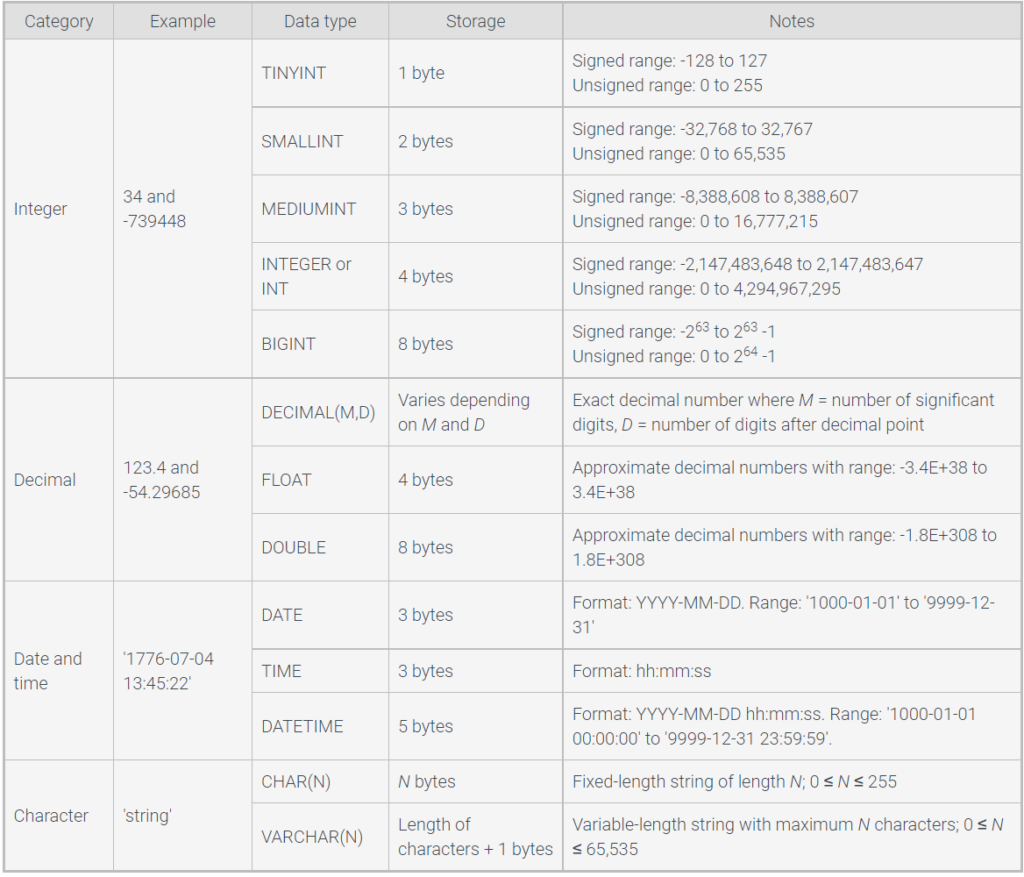
• Integer data types represent positive and negative integers. Several integer data types exist, varying by the number of bytes allocated for each value. Common integer data types include INT, implemented as 4 bytes of storage, and SMALLINT, implemented as 2 bytes.
• Decimal data types represent numbers with fractional values. Decimal data types vary by number of digits after the decimal point and maximum size. Common decimal data types include FLOAT and DECIMAL.
• Character data types represent textual characters. Common character data types include CHAR, a fixed string of characters, and VARCHAR, a string of variable length up to a specified maximum size.
• Time data types represent date, time, or both. Some time data types include a time zone or specify a time interval. Some time data types represent an interval rather than a point in time. Common time data types include DATE, TIME, DATETIME, and TIMESTAMP.
• Binary data types store data exactly as the data appears in memory or computer files, bit for bit. The database manages binary data as a series of zeros and ones. Common binary data types include BLOB, BINARY, VARBINARY, and IMAGE.
• Spatial data types store geometric information, such as lines, polygons, and map coordinates. Examples include POLYGON, POINT, and GEOMETRY. Spatial data types are relatively new and consequently vary greatly across database systems.
• Document data types contain textual data in a structured format such as XML or JSON.

Structural rules

Tables obey three structural rules:

1. Tables are normalized — exactly one value exists in each cell.
2. No duplicate column names — duplicate column names are not allowed in one table. However, the same column name can appear in different tables.
3. No duplicate rows — no two rows may have identical values in all columns.

In addition to the three rules, relational databases obey the principle of data independence,

which states that rows and columns of a table have no inherent order. 

1.3 Null values

NULL

NULL is a special value that represents missing data. 

NULL arithmetic and comparisons

An operator is a symbol that computes a value from one or more other values, called operands. The SQL language has several types of operators:

• Arithmetic operators, such as +, -, *, and /, compute numeric values from numeric operands.
• Comparison operators, such as <, >, and =, compute logical values TRUE or FALSE. Operands may be numeric, character, and other data types.
• Logical operators, AND, OR, and NOT, compute logical values from logical operands.

Whenever arithmetic or comparison operators have one or more NULL operands, the result is NULL. The key words IS NULL return true when compared to NULL and are used instead of = to select rows with NULLs.

NULL and aggregate functions

SQL statements also contain aggregate functions. An aggregate function operates on numeric values from multiple rows, including only rows selected by the WHERE clause. Aggregate functions include:

• SUM, which returns the total of selected values.
• AVG, which returns the average of selected values.
• MAX, which returns the largest selected value.
• MIN, which returns the smallest selected value.

SUM, AVG, MIN, and MAX ignore NULL values.

1.4 Primary and foreign keys

Primary keys

A primary key is a column, or group of columns, used to identify a row. 

Composite primary keys

Sometimes multiple columns are necessary to identify a row. A simple primary key consists of a single column. A composite primary key consists of multiple columns. 

In a minimal primary key, all columns are necessary for uniqueness.

Foreign keys

A foreign key is a column, or group of columns, that refer to a primary key.

1.5 Referential integrity

Referential integrity rules

A fully NULL foreign key is a simple or composite foreign key in which all columns are NULL. Referential integrity requires that all foreign key values must either be fully NULL or match some primary key value.

Referential integrity violations

Referential integrity can be violated in four ways:

1. A primary key is updated.
2. A foreign key is updated.
3. A row containing a primary key is deleted.
4. A row containing a foreign key is inserted.

Referential integrity actions

Databases can automatically correct referential integrity violations with any of four actions, which are specified in SQL when creating a table with a foreign key:

• RESTRICT rejects an insert, update, or delete that violates referential integrity.
• SET NULL sets invalid foreign keys to NULL.
• SET DEFAULT sets invalid foreign keys to a default primary key value, specified in SQL.
• CASCADE propagates primary key changes to foreign keys.

1.6 Normal form

Redundancy and dependence

Redundancy is the repetition of related values in a table. 

Normal forms

Normal forms are rules for designing tables with less redundancy. 

Dependence of one column on another is formally called functional dependence.

Multivalued dependence and join dependence entail dependencies between three or more columns.

First normal form

A table is in first normal form when all non-key columns depend on the primary key.

Second normal form

A table is in second normal form when all non-key columns depend on the whole primary key. 

Third normal form

Redundancy can occur in a second normal form table when a non-key column depends on another non-key column. Informally, a table is in third normal form when all non-key columns depend on the key, the whole key, and nothing but the key.

A candidate key is a simple or composite column that is unique and minimal. Minimal means all columns are necessary for uniqueness.

A non-key column is a column that is not contained in a candidate key.

A table is in third normal form if, whenever a non-key column A depends on column B, then B is unique. 

Boyce-Codd normal form

The definition of third normal form applies to non-key columns only, which allows for occasional redundancy. Boyce-Codd normal form applies to all columns and eliminates this redundancy.

A table is in Boyce-Codd normal form if, whenever column A depends on column B, then B is unique. Columns A and B may be simple or composite. This definition is identical to the definition of third normal form with the term ‘non-key’ removed.

2.1 Introduction to SQL

Structured Query Language

Structured Query Language (SQL) is a high-level computer language for storing, manipulating, and retrieving data in a relational database. 

SQL syntax

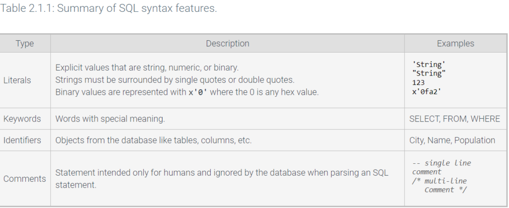
An SQL statement is a complete command composed of one or more clauses. A clause groups SQL keywords like SELECT, FROM, and WHERE with table names like City, column names like Name, and conditions like Population > 100000.

SQL sublanguages

The SQL language is divided into five sublanguages:

• Data Definition Language (DDL) defines the structure of the database.
• Data Query Language (DQL) retrieves data from the database.
• Data Manipulation Language (DML) manipulates data stored in a database.
• Data Control Language (DCL) controls database user access.
• Data Transaction Language (DTL) manages database transactions.

2.2 Creating and dropping databases

CREATE DATABASE and DROP DATABASE statements

The CREATE DATABASE statement creates a new database. Once a database is created, tables can be added to the database. The DROP DATABASE statement deletes the database, including all tables in the database.

SHOW statement

The SHOW statement provides database users and administrators with information about databases, the database contents (tables, columns, etc.), and server status information.

Commonly used SHOW statements include:

• SHOW DATABASES lists databases available in the database system.
• SHOW TABLES lists tables available in the currently selected database.
• SHOW COLUMNS lists columns available in a specific table named by a FROM clause.
• SHOW CREATE TABLE shows the CREATE TABLE statement for a given table.

The USE statement selects a database and is required to show information about tables within a specific database.

2.3 Creating and dropping tables

SQL data types

When creating a table, every table column must be assigned a data type. Common data types include: integer, decimal, date and time, and character. Most databases allow integer and decimal numbers to be signed or unsigned.

• A signed number is a number that may be negative.
• An unsigned number is a number that cannot be negative.

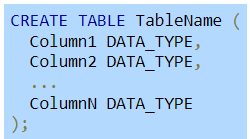
CREATE TABLE and DROP TABLE statements

The CREATE TABLE statement creates a new table by specifying the table name, column names, and column data types.

Figure 2.3.1: CREATE TABLE syntax.

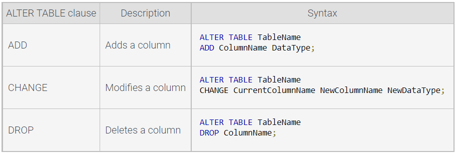
ALTER TABLE statement

The ALTER TABLE statement adds, deletes, or modifies columns on an existing table. 

Table 2.3.2: ALTER TABLE ADD, CHANGE, and DROP syntax.

2.4 Primary and foreign key constraints

PRIMARY KEY constraint

A constraint is a rule that applies to table data. Constraints are specified in a CREATE TABLE statement or may be added to a preexisting table with an ALTER TABLE statement.

The PRIMARY KEY constraint in a CREATE TABLE statement names the table’s primary key, the column(s) that uniquely identify each row.

Auto-increment columns

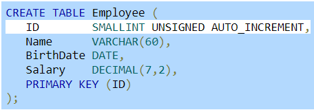
A primary key on an ID column is commonly implemented as an auto-increment column. An auto-increment column is a column that is assigned an automatically incrementing value.

The AUTO_INCREMENT keyword defines an auto-increment column in MySQL.

Figure 2.4.1: ID is an AUTO_INCREMENT column.

FOREIGN KEY constraint

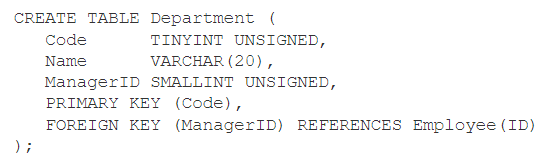
A foreign key constraint is added to a CREATE TABLE statement with the FOREIGN KEY and REFERENCES keywords. 

ON DELETE and ON UPDATE actions

Actions can be specified on the FOREIGN KEY constraint with ON DELETE and ON UPDATE keywords:

• ON DELETE responds to an invalid primary key deletion. Ex: Deleting a primary key 1234 that is used in a foreign key.
• ON UPDATE responds to an invalid primary key update. Ex: Updating a primary key 1234 to 5555 when 1234 is used in a foreign key.

ON DELETE and ON UPDATE must be followed by a response:

• RESTRICT rejects an insert, update, or delete that violates referential integrity. RESTRICT is applied by default when no action is specified.
• SET NULL sets an invalid foreign key value to NULL.
• SET DEFAULT sets invalid foreign keys to a default primary key value.
• CASCADE propagates primary key changes to foreign keys. If a primary key is deleted, rows containing matching foreign keys are deleted. If a primary key is updated, matching foreign keys are updated to the same value.

2.5 Column constraints

NOT NULL constraint

 The NOT NULL constraint is used in a CREATE TABLE statement to prevent a column from having a NULL value.

DEFAULT constraint

When a row is inserted into a table, an unspecified value is assigned NULL by default. The DEFAULT constraint is used in a CREATE TABLE statement to specify a column’s default value when no value is provided.

UNIQUE constraint

A table’s primary key always has unique values, but values in other columns may contain duplicates. The UNIQUE constraint ensures that all column values are unique.

The UNIQUE constraint may be applied to a single column or to multiple columns. A constraint that is applied to a single column is called a column-level constraint. A constraint that is applied to multiple columns is called a table-level constraint.

CHECK constraint

The CHECK constraint specifies an expression that limits the range of a column’s values. 

BETWEEN operator

Determining if a value is between two other values, like the animation above does with HireDate, is a common SQL operation. The BETWEEN operator provides an alternative way to determine if a value is between two other values. Ex:

-- Same as: HireDate >= '2000-01-01' AND HireDate <= '2020-01-01'
HireDate DATE CHECK (HireDate BETWEEN '2000-01-01' AND '2020-01-01'),

CONSTRAINT keyword

MySQL gives constraints a default name if no name is specified. A constraint can be given a name using the CONSTRAINT keyword, followed by the constraint name and declaration. 

2.6 Inserting, updating, and deleting rows

INSERT statement

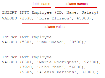
The INSERT statement adds rows to a table. The INSERT statement includes the INTO and VALUES clauses:

• The INTO clause names the table and columns where data is to be added.
• The VALUES clause specifies the column values to be added.

UPDATE statement

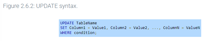
The UPDATE statement modifies existing rows in a table. The UPDATE statement uses the SET clause to specify the new column values.

The UPDATE statement uses a WHERE clause to determine which rows are updated. The WHERE clause is used with UPDATE, DELETE, and SELECT statements to specify a condition that must be true for a row to be chosen. Omitting the WHERE clause results in all rows being updated.

DELETE statement

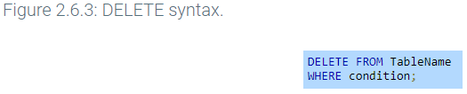
The DELETE statement deletes existing rows in a table. The FROM keyword is followed by the table name whose rows are to be deleted. The WHERE clause specifies which rows should be deleted. Omitting the WHERE clause results in all rows in the table being deleted.

TRUNCATE

The TRUNCATE statement deletes all rows from a table. TRUNCATE is nearly identical to a DELETE statement with no WHERE clause except for some small differences that depend on the database system. Ex: In MySQL, A TRUNCATE statement resets the table’s auto-increment values back to 1, but a DELETE statement does not.

TRUNCATE TABLE TableName;

2.7 Selecting rows

SELECT statement

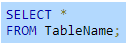
The SELECT statement selects rows from a table named in the FROM clause. The data returned from the SELECT statement, called the result set, is stored in a result table. Column names are listed after the SELECT keyword, separated by commas. The columns names can be replaced with an asterisk (*) to select all columns.

Figure 2.7.1: SELECT syntax.

Figure 2.7.2: SELECT all columns.

Long tables

Some tables may contain thousands or millions of rows, and selecting all rows can take a long time. MySQL has a LIMIT clause that limits the number of rows returned by a SELECT statement. Ex: The SELECT statement below returns only the first 100 rows from the City table.

WHERE clause

The SELECT statement retrieves all rows by default. The WHERE clause is combined with the SELECT statement to filter the result set. The WHERE clause must come after the FROM clause.

Figure 2.7.3: SELECT FROM WHERE syntax.

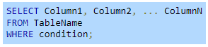
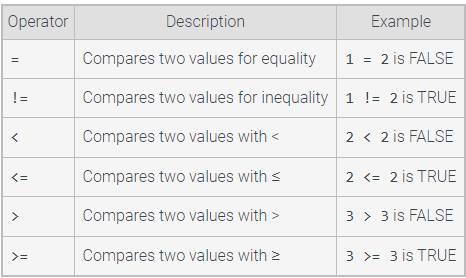
The WHERE clause works like an if statement in a programming language, specifying conditions that must be true for a row to be selected. A condition is an expression that evaluates to TRUE, FALSE, or NULL. Only a condition that is TRUE selects the row. A condition uses a comparison operator to compare two values. Common comparison operators are summarized in the table below.

Table 2.7.1: Common comparison operators.

Logical operators

The WHERE clause supports logical operators AND, OR, and NOT. A logical operator evaluates to TRUE, FALSE, or NULL. Ex: 1 < 2 AND 2 < 3 is TRUE because the condition on the left is TRUE, and the condition on the right is TRUE

Arithmetic operators

The SELECT statement supports arithmetic operators, which perform calculations on two operands. Arithmetic operators can be used in the SELECT clause or the WHERE clause.

DISTINCT clause

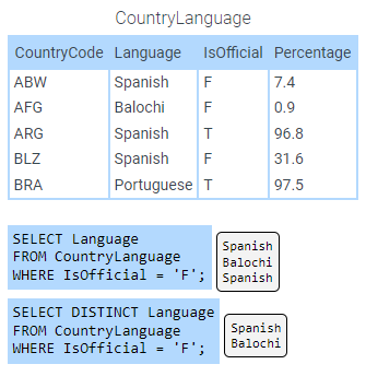
The DISTINCT clause is used with a SELECT statement to return only unique or ‘distinct’ values.

Figure 2.8.1: SELECT DISTINCT example.

IN operator

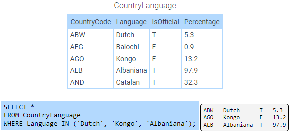
The IN operator is used in a WHERE clause to determine if a value matches one of several values. The SELECT statement in the figure below uses the IN operator to select only rows where the Language column has a Dutch, Kongo, or Albaniana value.

Figure 2.8.2: Using the IN operator.

LIKE operator

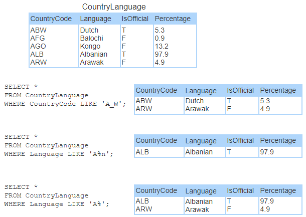
The LIKE operator, when used in a WHERE clause, matches text against a pattern using the two wildcard characters % and _.

• % matches any number of characters. Ex: LIKE 'L%t' matches “Lt”, “Lot”, “Lift”, and “Lol cat”.
• _ matches exactly one character. Ex: LIKE 'L_t' matches “Lot” and “Lit” but not “Lt” and “Loot”.

The LIKE operator performs case-insensitive pattern matching by default or case-sensitive pattern matching if followed by the BINARY keyword. Ex: LIKE BINARY 'L%t' matches ‘Left’ but not ‘left’.

To search for the wildcard characters % or _, a backslash (\) must precede % or _. Ex: LIKE 'a\%' matches “a%”.

ORDER BY clause

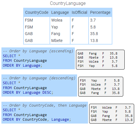
A SELECT statement selects rows from a table with no guarantee the data will come back in a certain order. The ORDER BY clause orders selected rows by one or more columns in ascending (alphabetic or increasing) order. The DESC keyword with the ORDER BY clause orders rows in descending order.

SAMPLE CODE:

CREATE TABLE Song (
ID INT,
Title VARCHAR(60),
Artist VARCHAR(60),
ReleaseYear INT,
PRIMARY KEY (ID)
);

INSERT INTO Song VALUES
(100, ‘Hey Jude’, NULL, 1968),
(200, ‘When Doves Cry’, ‘Prince’, 1997),
(300, NULL, ‘The Righteous Brothers’, 1964),
(400, ‘Johnny B. Goode’, ‘Chuck Berry’, 1958),
(500, ‘Smells Like Teen Spirit’, NULL, 1991),
(600, NULL, ‘Aretha Franklin’, 1967);

— Modify the SELECT statement
SELECT *
FROM Song;

3.1 Functions

Aggregate functions

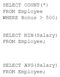
MySQL has functions for processing strings, numbers, dates, and times. An aggregate function is a function that works on a group of values. Some common aggregate functions include:

• COUNT() – Counts the number of rows retrieved by a SELECT statement.
• MIN() – Finds the minimum value in a group.
• MAX() – Finds the maximum value in a group.
• SUM() – Sums all the values in a group.
• AVG() – Finds the arithmetic mean (average) of all the values in a group.

GROUP BY and HAVING clauses

Aggregate functions are commonly used with the GROUP BY clause. The GROUP BY clause groups rows with identical values into a set of summary rows. Some important points about the GROUP BY clause:

The HAVING clause is used with the GROUP BY clause to filter group results. The HAVING clause must appear after the GROUP BY clause but before the optional ORDER BY clause.

Numeric functions

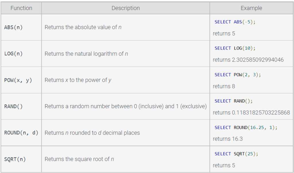
SQL numeric functions perform useful calculations beyond simple addition, subtraction, multiplication, and division.

Table 3.1.1: Common numeric functions.

String functions

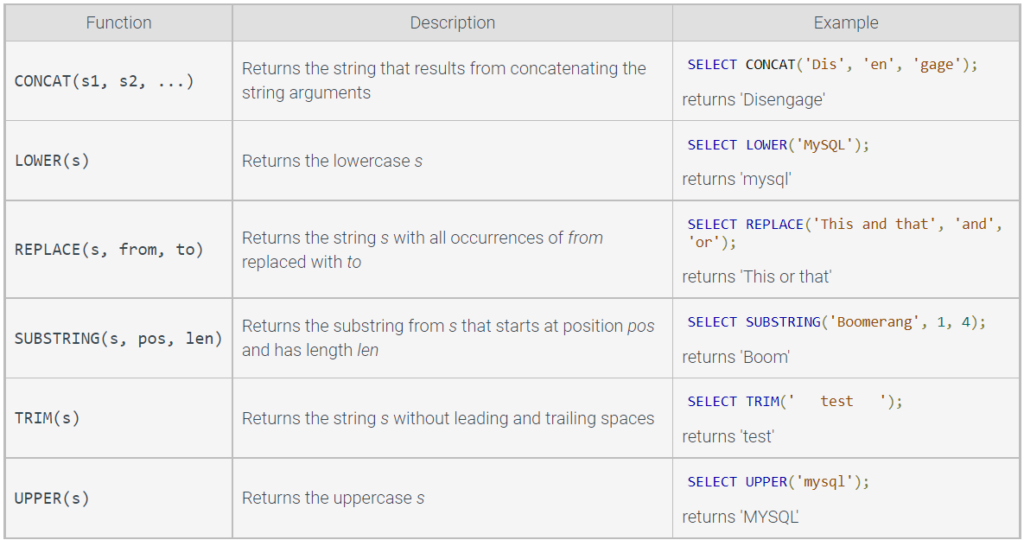
SQL string functions manipulate strings. Some common string functions are summarized in the table below.

Table 3.1.2: Common string functions.

Date and time functions

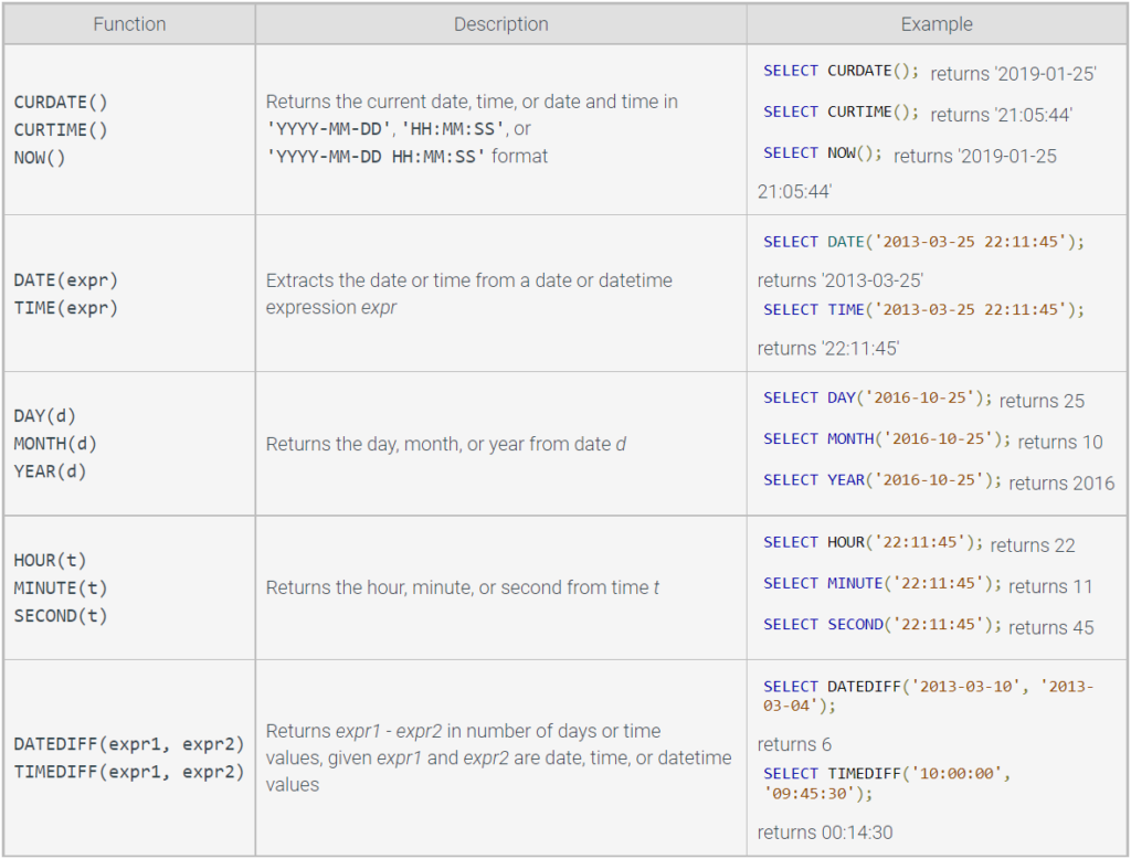
Date and time functions operate on DATE, TIME, and DATETIME data types.

Table 3.1.3: Common date and time functions.

3.2 Inner and outer joins

Joins

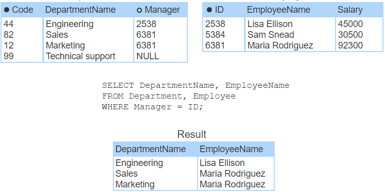
In relational databases, reports are commonly generated from data in multiple tables. Multi-table reports are written with join statements.

A join is a SELECT statement that combines data from two tables, known as the left table and right table, into a single result. The tables are combined by comparing columns from the left and right tables, usually with the = operator. The columns must have comparable data types.

Usually, a join compares a foreign key of one table to the primary key of another. However, a join can compare any columns with comparable data types.

Left and right joins

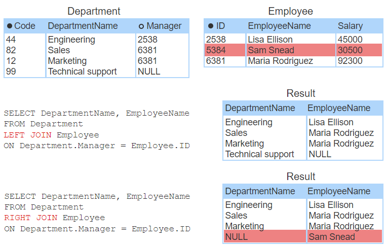
In some cases, the database user wants to see unmatched rows from either the left or right table, but not both. To enable these cases, relational databases support left and right joins:

• LEFT JOIN selects all left table rows, but only matching right table rows.
• RIGHT JOIN selects all right table rows, but only matching left table rows.

An outer join is any join that selects unmatched rows, including left, right, and full joins.

Join clauses are standard SQL syntax and supported by most relational databases. MySQL supports INNER, LEFT, and RIGHT JOIN but not FULL JOIN. For details of MySQL join syntax, see the link in ‘Exploring further’ below.

Special cases

Relational databases have several special joins. Most special joins are used infrequently for unusual reporting needs. All of the following special joins can be implemented as an inner, left, right, or full join:

An equijoin compares columns of two tables with the = operator. Most joins are equijoins, including the examples above.

A non-equijoin compares columns with an operator other than =, such as <, >. In the example below, a non-equijoin selects all buyers along with properties priced below the buyer’s maximum price.

In a self-join, a table is joined to itself. A self-join can compare any columns of a table, as long as the columns have comparable data types. If a foreign key and the referenced primary key are in the same table, a self-join might compare key columns.

In a self-join, aliases are necessary to distinguish left and right tables. An alias is a temporary name assigned to a column or table. In the example below, A is the left table’s alias, and B is the right table’s alias. A.Name is the Name column of the left table, representing the employee. B.Name is the Name column of the right table, representing the employee’s manager. The result shows employees along with each employee’s manager.

A cross-join combines two tables without comparing columns. A cross-join uses the CROSS JOIN keywords without a WHERE or ON clause. As a result, all possible combinations of rows from both tables appear in the result.

3.3 Subqueries

Subqueries

A subquery, sometimes called a nested query or inner query, is a query within another SQL query. The subquery is typically used in a SELECT statement’s WHERE clause to return data to the outer query and restrict the selected results. The subquery is placed inside parentheses ().

Correlated subqueries

A subquery is correlated when the subquery’s WHERE clause references a column from the outer query. In a correlated subquery, the rows selected depend on what row is currently being examined by the outer query.

An alias can also help differentiate the columns. An alias is a temporary name assigned to a column or table. The AS keyword follows a column or table name to create an alias. Ex: SELECT Name AS N FROM Country AS C creates the alias N for the Name column and alias C for the Country table. The AS keyword is optional and may be omitted. Ex: SELECT Name N FROM Country C.

EXISTS operator

Correlated subqueries commonly use the EXISTS operator, which returns TRUE if a subquery selects at least one row and FALSE if no rows are selected. The NOT EXISTS operator returns TRUE if a subquery selects no rows and FALSE if at least one row is selected.

3.5 View tables

Creating views

Table design is optimized for a variety of reasons, such as minimal storage, fast query execution, and support for structural and business rules. Occasionally, the design is not ideal for database users and programmers. 

A view table is a table name associated with a SELECT statement, called the view query. The CREATE VIEW statement creates a view table and specifies the view name, query, and, optionally, column names. If column names are not specified, column names are the same as in the view query result table.

Figure 3.5.1: CREATE VIEW statement.

Querying views

A table specified in the view query’s FROM clause is called a base table. Unlike base table data, view table data is not normally stored. Instead, when a view table appears in an SQL statement, the view query is merged with the SQL query. The database executes the merged query against base tables.

In some databases, view data can be stored. A materialized view is a view for which data is stored at all times. Whenever a base table changes, the corresponding view tables can also change, so materialized views must be refreshed. To avoid the overhead of refreshing views, MySQL and many other databases do not support materialized views.

Querying views

A table specified in the view query’s FROM clause is called a base table. Unlike base table data, view table data is not normally stored. Instead, when a view table appears in an SQL statement, the view query is merged with the SQL query. The database executes the merged query against base tables.

In some databases, view data can be stored. A materialized view is a view for which data is stored at all times. Whenever a base table changes, the corresponding view tables can also change, so materialized views must be refreshed. To avoid the overhead of refreshing views, MySQL and many other databases do not support materialized views.

Advantages of views

View tables have several advantages:

• Protect sensitive data. A table may contain sensitive data. Ex: The Employee table contains compensation columns such as Salary and Bonus. A view can exclude sensitive columns but include all other columns. Authorizing users and programmers access to the view but not the underlying table protects the sensitive data.
• Save complex queries. Complex or difficult SELECT statements can be saved as a view. Database users can reference the view without writing the SELECT statement.
• Save optimized queries. Often, the same result table can be generated with equivalent SELECT statements. Although the results of equivalent statements are the same, performance may vary. To ensure fast execution, the optimal statement can be saved as a view and distributed to database users.

Updating views

View tables are commonly used in SELECT statements. Using views in INSERT, UPDATE, and DELETE statements is problematic:

• Primary keys. If a base table primary key does not appear in a view, an insert to the view generates a NULL primary key value. Since primary keys may not be NULL, the insert is not allowed.
• Aggregate values. A view query may contain aggregate functions such as AVG() or SUM(). One aggregate value corresponds to many base table values. An update or insert to the view may create a new aggregate value, which must be converted to many base table values. The conversion is undefined, so the insert or update is not allowed.
• Join views. In a join view, foreign keys of one base table may match primary keys of another. A delete from a view might delete foreign key rows only, or primary key rows only, or both the primary and foreign key rows. The effect of the join view delete is undefined and therefore not allowed.

WITH CHECK OPTION clause

Databases that allow view updates face one particularly bothersome behavior. A view insert or update may create a row that does not satisfy the view query WHERE clause. In this case, the inserted or updated row does not appear in the view table. From the perspective of the database user, the insert or update appears to fail even though the base tables have changed.

To prevent inserts or updates that appear to fail, databases that support view updates have an optional WITH CHECK OPTION clause. When WITH CHECK OPTION is specified, the database rejects inserts and updates that do not satisfy the view query WHERE clause. Instead, the database generates an error message that explains the violation.

Figure 3.5.2: WITH CHECK OPTION clause.

Final So Far:

CREATE TABLE COFFEE_SHOP (
shop_id INT PRIMARY KEY,
shop_name VARCHAR(50),
city VARCHAR(50),
state CHAR(2)
);

CREATE TABLE SUPPLIER (
supplier_id INT PRIMARY KEY,
company_name VARCHAR(50),
country VARCHAR(30),
sales_contact_name VARCHAR(60),
email VARCHAR(50) NOT NULL
);

CREATE TABLE EMPLOYEE (
employee_ID INT PRIMARY KEY,
first_name VARCHAR(30),
last_name VARCHAR(30),
hire_date DATE,
job_title VARCHAR(30),
shop_id INT,
FOREIGN KEY (shop_id) REFERENCES COFFEE_SHOP(shop_id)
);

CREATE TABLE COFFEE (
coffee_id INT PRIMARY KEY,
shop_id INT,
supplier_id INT,
coffee_name VARCHAR(30),
price_per_pound NUMERIC(5,2),
FOREIGN KEY (supplier_id) REFERENCES SUPPLIER(supplier_id),
FOREIGN KEY (shop_id) REFERENCES COFFEE_SHOP(shop_id)
);

INSERT INTO COFFEE_SHOP VALUES
(001,”Sparkys”,”Springfield”,”OR”),
(002,”Joes Cup”,”Seattle”,”WA”),
(003,”Caffie Cafe”,”Portland”,”OR”);

INSERT INTO SUPPLIER VALUES
(3548,”Syscom”,”Colombia”,”Maria Zabeo”, “mzabeo@syscom.co”),
(8276,”RaviBella”, “Brazil”, “Neymar Costa”, “Neycosta@ravibella.br”),
(1435,”Banh Xe”, “Vietnam”, “Hanh Nguyen”, “nguyen.hanh@banhxe.vn”);

INSERT INTO EMPLOYEE VALUES
(132, “John”, “Ferdinand”, “2020-08-05”, “Barista”, 001),
(155, “Autumn”, “Howard”, “2021-03-03”, “Clerk”, 003),
(093, “Beth”, “Lewis”, “2018-12-01”, “Store Manager”, 001);

INSERT INTO COFFEE VALUES
(234, 002, 8276, “Kama Sumatra”, 028.99),
(235, 001, 1435, “Musta Robusta”, 019.99),
(236, 003, 3548, “Mars Volcanica”, 024.99);

ALTER TABLE EMPLOYEE ADD COLUMN employee_full_name VARCHAR(200);

UPDATE EMPLOYEE SET employee_full_name = CONCAT(first_name, ” “, last_name);

CREATE INDEX coffee_index ON COFFEE (Coffee_name);

SELECT * FROM EMPLOYEE;

SELECT * FROM COFFEE_SHOP
WHERE state = “OR”;

SELECT COFFEE.coffee_name, SUPPLIER.country, COFFEE.price_per_pound, COFFEE_SHOP.shop_name, COFFEE_SHOP.city
FROM COFFEE
INNER JOIN SUPPLIER
on COFFEE.supplier_id = SUPPLIER.supplier_id
INNER JOIN COFFEE_SHOP
on COFFEE.shop_id = COFFEE_SHOP.shop_id;

4.1 MySQL

MySQL

This material uses MySQL as a reference relational database system. MySQL is a leading relational database system sponsored by Oracle. 

The latest MySQL release is 8.0, available in two editions:

• MySQL Community, commonly called MySQL Server, is a free edition. MySQL Server includes a complete set of database services and tools, and is suitable for non-commercial applications such as education.
• MySQL Enterprise is a paid edition for managing commercial databases. MySQL Enterprise includes MySQL Server and additional administrative applications.

Instructions for downloading and installing MySQL Server on Windows or Mac OS are available from the ‘Exploring further’ links below.

When installing MySQL Server, the user must enter a password for the root account, the administrative account that has full control of MySQL. 

MySQL Command-Line Client

The MySQL Command-Line Client is a text interface included in the MySQL Server download

MySQL Server returns an error code and description when an SQL statement is syntactically incorrect or the database cannot execute the statement.

MySQL Workbench

Some developers prefer to interact with MySQL Server via a graphical user interface. MySQL Workbench is installed with MySQL Server and allows developers to execute SQL commands using an editor.

The figure below shows the MySQL Workbench home screen on Windows. The Mac version has some minor differences. Clicking on the box labeled Local Instance MySQL80 connects to MySQL Server running on the same computer as MySQL Workbench.

After connecting to MySQL server, Workbench shows the Navigator sidebar on the left with two tabs:

1. The Administration tab shows various administrative options, like checking the server’s status, importing/exporting data, and starting/stopping the MySQL server.
2. The Schemas tab shows a list of available databases. A database can be expanded to show the database’s tables.

4.2 MySQL architecture

Layers

Architecture describes the components of a computer system and the relationships between components. This section describes MySQL architecture. Other relational databases have similar components, but component details and relationships vary greatly.

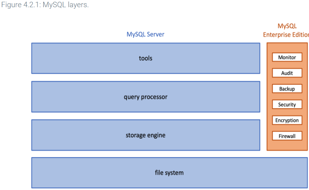
MySQL components are organized in four layers:

• Tools interact directly with database users and administrators, and send queries to the query processor.
• The query processor manages connections from multiple users and compiles queries into low-level instructions for the storage engine.
• The storage engine executes instructions, manages indexes, and interacts with the file system. Some storage engines support database transactions, described elsewhere in this material.
• The file system contains system and user data, such as log files, tables, and indexes.

MySQL is available in a free version, called MySQL Server, and a paid version, called MySQL Enterprise Edition. The Enterprise Edition includes MySQL Server and components for high-end commercial installations, such as:

• Monitor collects and displays information on CPU, memory, and index utilization, as well as queries and results. Database administrators use Enterprise Monitor to manage and tune large databases with many users.
• Audit keeps track of all database changes. For each change, Audit tracks the time of change and who made the change. Audit supports government and business audit requirements for sensitive databases such as financial, medical, and defense.

Tools

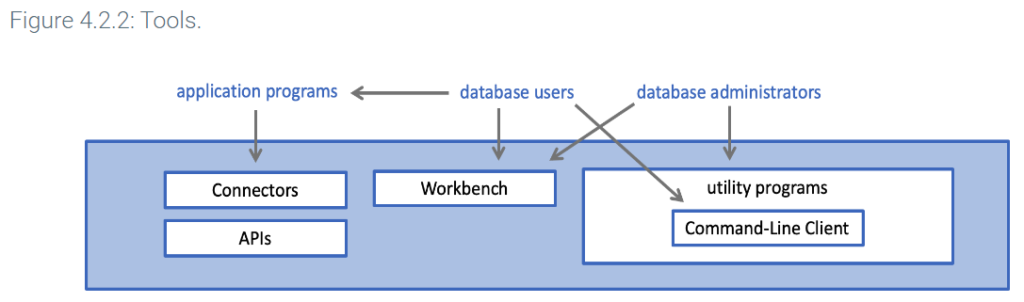
The tools layer includes Connectors and APIs, Workbench, and utility programs.

Utility programs include approximately 30 tools, grouped in five categories: installation, client, administrative, developer, and miscellaneous tools. Most utility programs are intended for database administrators or programmers. Example functions include:

• Upgrade existing databases to a new MySQL release
• Backup databases
• Import data to databases
• Inspect log files
• Administer database servers

The Command-Line Client is a particularly important utility program, commonly used by both database administrators and users. The Command-Line Client displays the mysql> prompt and processes individual SQL queries interactively.

Query processor

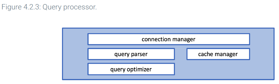
The query processor layer has two main functions: manage connections and compile queries.

A connection is a link between tools and the query processor. Each connection specifies a database name, server address, logon name, and password. The connection manager creates connections and manages communications between tools and the query parser.

Query compilation generates a query execution plan. An execution plan is a detailed, low-level sequence of steps that specify exactly how to process a query.

The query processor generates an execution plan in two steps:

1. The query parser checks each query for syntax errors and converts valid queries to an internal representation.
2. The query optimizer reads the internal representation, generates alternative execution plans, estimates execution times, and selects the fastest plan. Estimates are based on heuristics and statistics about data, like the number of rows in each table and the number of values in each column. These statistics are maintained in the data dictionary, described below.

For optimal performance, the query processor layer has a cache manager that stores reusable information in main memory. Ex: The cache manager retains execution plans for queries that are submitted multiple times. If data used in repeated queries does not change, the cache manager may also save query results.

Storage engine

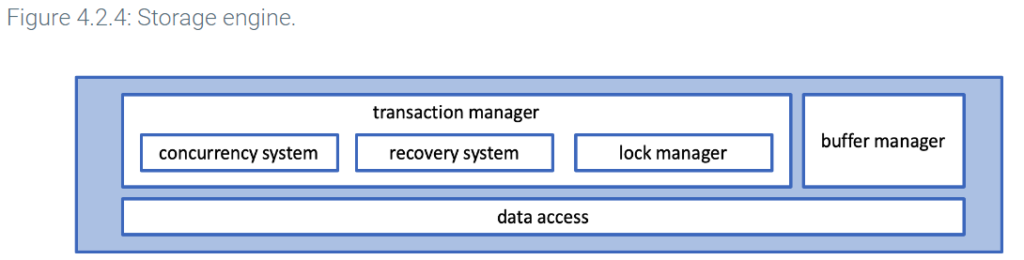
The storage engine layer has two main functions: transaction management and data access.

To reduce data access time, the buffer manager retains data blocks from the file system for possible reuse. The data blocks are retained in an area of main memory called the buffer. Ex: If queries frequently access department data, the buffer manager may retain some or all blocks of the Department table. The buffer manager is similar to the cache manager of the query processor layer.

The buffer manager has a fixed amount of memory. As the database processes queries and reads blocks, an algorithm determines which blocks to retain and which to discard. The InnoDB buffer manager uses a least recently used or LRU algorithm.

Most databases do not offer configurable storage engines and use the term storage manager instead of storage engine.

File system

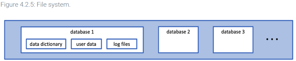
The file system layer consists of data stored on storage media and organized in files. The file system contains three types of data for each database: user data, log files, and a data dictionary.

A catalog, also known as a data dictionary, is a directory of tables, columns, keys, indexes, and other objects in a relational database. All relational databases contain a catalog. Query processors and storage managers use catalog information when queries are processed and executed.

MySQL uses the term ‘data dictionary’. The MySQL data dictionary contains roughly 30 tables, including:

• tables describes all tables
• table_stats contains table statistics, such as the number of rows in each table
• columns describes all columns
• foreign_keys describes all foreign keys
• indexes describes all indexes
• routines describes all stored procedures and stored functions
• triggers describes all triggers

Data dictionary tables cannot be accessed directly with SELECT, INSERT, UPDATE, and DELETE queries. However, the table contents can be accessed indirectly. The SHOW query is compiled as a SELECT query against dictionary tables. Ex: SHOW COLUMNS generates a SELECT query against the columns table. CREATE generates an INSERT, ALTER generates an UPDATE, and DROP generates a DELETE against dictionary tables.

5.1 Entities, relationships, and attributes

The entity-relationship model

Database design begins with verbal or written requirements for the database. Requirements are formalized as an entity-relationship model and then implemented in SQL.

An entity-relationship model is a high-level representation of data requirements, ignoring implementation details. An entity-relationship model guides implementation in a particular database system, such as MySQL.

An entity-relationship model includes three kinds of objects:

• An entity is a person, place, product, concept, or activity.
• A relationship is a statement about two entities.
• An attribute is a descript­ive property of an entity.

Entity-relationship diagram and glossary

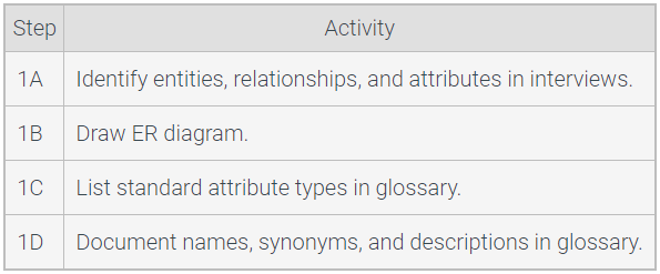
An entity-relationship diagram, commonly called an ER diagram, is a schematic picture of entities, relationships, and attributes. Entities are drawn as rectangles. Relationships are drawn as lines connecting rectangles. Attributes appear as additional text within an entity rectangle, under the entity name.

A glossary, also known as a data dictionary or repository, documents additional detail in text format. A glossary includes names, synonyms, and descriptions of entities, relationships, and attributes. For simple databases with few users, a database designer may record the glossary with a text editor. For more complex databases, the designer may use a database or software tool specifically designed for glossaries.

Types and instances

In entity-relationship modeling, a type is a set:

• An entity type is a set of things. Ex: All employees in a company.
• A relationship type is a statement about entity types. Ex: Employee-Manages-Department.
• An attribute type is a set of values. Ex: All employee salaries.

Entity, relationship, and attribute types usually become tables, foreign keys, and columns, respectively.

An instance is an element of a set:

• An entity instance is an individual thing. Ex: The employee Sam Snead.
• A relationship instance is a statement about entity instances. Ex: “Maria Rodriguez manages Sales.”
• An attribute instance is an individual value. Ex: The salary $35,000.

Database design

Complex databases are developed in three phases:

1. Analysis develops an entity-relationship model, capturing data requirements while ignoring implementation details.
2. Logical design converts the entity-relationship model into tables, columns, and keys for a particular database system.
3. Physical design adds indexes and specifies how tables are organized on storage media.

5.2 Binary relationships

What is a binary relationship?

The simplest kind of relationship is known as a binary relationship. 

Cardinality

One‐to‐one binary relationship

Figure 5.2.2 shows three binary relationships of different cardinalities, representing the maximum number of entities that can be involved in a particular relationship

One‐to‐many binary relationship

Associations can also be multiple in nature. Figure 5.2.2b shows a one‐to‐many (1‐M) binary relationship between salespersons and customers. 

Many‐to‐many binary relationship

Figure 5.2.2c shows a many‐to‐many (M‐M) binary relationship among salespersons and products. A salesperson is authorized to sell many products; a product can be sold by many salespersons. 

Modality

Figure 5.2.3 shows the addition of the modality, the minimum number of entity occurrences that can be involved in a relationship. I

More about many‐to‐many relationships

Intersection data

Generally, we think of attributes as facts about entities.

It describes the combination of or the association between that particular salesperson and that particular product and it is known as intersection data. 

Associative entity

Since we know that entities can have attributes and now we see that many‐to‐many relationships can have attributes, too, does that mean that entities and many‐to‐many relationships can in some sense be treated in the same way within E‐R diagrams? Indeed they can! Figure 5.2.5 shows the many‐to‐many relationship Sells converted into the associative entity SALES. 

5.5 Discovery

Discovery

Entities, relationships, and attributes are discovered in interviews with database users and managers. 

Names

Entity names are a singular noun. Ex: Employee rather than Employees. The best names are commonly used and easily understood by database users.

Relationships names have the form Entity-Verb-Entity, such as Division-Contains-Department. When the related entities are obvious, in ER diagrams or informal conversation, Verb is sufficient and entity names can be omitted. The verb should be active rather than passive. Ex: Manages rather than IsManagedBy. Occasionally, the same verb relates different entity pairs. Ex: Order-Contains-LineItem and Division-Contains-Department.

Attribute names have the form EntityQualifierType, such as EmployeeFirstName:

• Entity is the name of the entity that the attribute describes. When the entity is obvious, in ER diagrams or informal conversation, QualifierType is sufficient and the entity name can be omitted.
• Qualifier describes the meaning of the attribute. Ex: First, Last, and Alternate. Sometimes a qualifier is unnecessary and can be omitted. Ex: StudentNumber.
• Type is chosen from a list of standard attribute types such as Name, Number, and Count. Attribute types are not identical to SQL data types. Ex: “Amount” might be an attribute type representing monetary values, implemented as the MONEY data type in SQL. “Count” might be an attribute type representing quantity, implemented as NUMBER in SQL.

Database design

The first step of the analysis phase is discovery of entities, relationships, and attributes in interviews and document review.