4.11 Lesson: Linear equations using an inverse matrix

• After completing this lesson you should be able to solve a system of linear equations using an inverse matrix.
• Solving matrix equations using inverse matrices

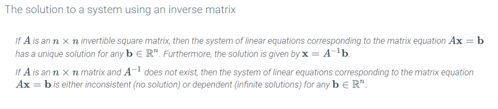
• Solve the system of equations by finding a vector x that satisfies the equation Ax=b.
  • If the coefficient matrix has an inverse, use it to solve the system.
    • Multiply the left-hand sides of both sides of the equation by A−1 (matrix A inverse.)
    • Using the associative property of matrix multiplication, A−1(Ax)=(A−1A)x
    • The product of A−1A=In(the Identity matrix.)
      Ax=bA−1(Ax)=A−1b(A−1A)x=A−1bIx=A−1bx=A−1b
  • If a square coefficient matrix has an inverse, then Ax=b has a unique solution for any b in Rn.
  • If a square coefficient matrix does not have an inverse, then the system Ax=b either has no solution or infinitely many solutions.

4.12 Lesson: Elementary matrix operations

• After completing this lesson you should be able to perform row operations on a square 2 x 2 or 3 x 3 matrix.
• Elementary row operations
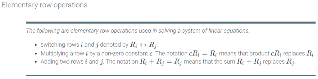
• Operations performed to obtain row-equivalent matrices are called elementary row operations.
• Matrices are row-equivalent if a sequence of elementary row operations exists that can transform one matrix into the other.

• Elementary matrices
• An elementary matrix is a matrix that represents an elementary row operation.

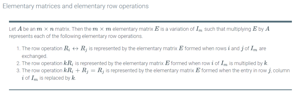
• An elementary matrix is the identity matrix with a row operation applied to it.
• There are three elementary row operations that can be performed on a matrix. The following is a description of the elementary row operations.

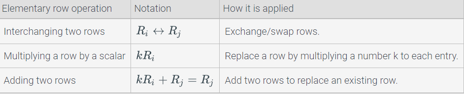
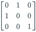
• Each row operation on a matrix A can be achieved by multiplying A by an elementary matrix. For example, if you want to interchange the first row of matrix A with the second row of matrix A, you would multiply A by the elementary matrix:

4.13 Lesson: Gaussian elimination

• After completing this lesson you should be able to perform Gaussian elimination on a given matrix equation.
• Echelon form
• A zero row is a row in a matrix that has no nonzero entries. 
• A nonzero row is a row in a matrix that has at least one nonzero entry and a nonzero column is a column in a matrix that has at least one nonzero entry.
• The leading entry of a row is the first nonzero entry from the left.

A matrix is in echelon form if the matrix has the following properties:

1. Any zero rows are below all nonzero rows.
2. The leading entry of each row is to the right of the leading entries in the rows above.
3. All the entries below a leading entry are zeros.

• Reduced echelon form

A matrix is in reduced echelon form if the matrix has the following properties:

1. Any rows that contain all zeros are below all nonzero rows.
2. The leading entry of each row is to the right of the leading terms in the rows above.
3. All the entries below a leading entry are zeros.
4. The leading entry for each nonzero row is 1.
5. Each leading entry of 1 has zeros above. That is, the leading ones are the only nonzero entry in that column.

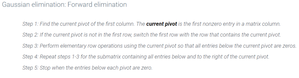
• Gaussian elimination: Forward elimination
• Gaussian elimination is an algorithm used to solve a system of linear equations.
• Forward elimination is the process of transforming a matrix that represents a system of linear equations into row echelon form.

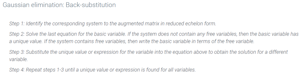
• Gaussian elimination: Back-substitution
• Back-substitution is the process of substituting the value of the last variable into each of the preceding equations to obtain the values of the remaining variables.

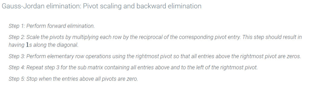
• Gauss-Jordan algorithm
• The Gauss-Jordan algorithm is an algorithm that transforms a matrix into reduced echelon form. 
• Pivot scaling is the process of transforming each pivot into 1.
• Backward elimination is the process of transforming a matrix that represents a system of linear equations from row echelon form to reduced echelon form.

• If a matrix B is obtained by performing a sequence of elementary row operations on a matrix A, then B and A are row equivalent.
• Gauss-Jordan elimination is an algorithm for getting matrices in reduced row echelon form.
• Echelon form is when all non-zero rows are above any rows of all zeros and the leading coefficient of any row is always to the right of the leading coefficient of any row above it.
• To construct a row equivalent matrix in echelon form, multiply the coefficient matrix A by a sequence of elementary matrices.

4.14 Lesson: Elementary matrices and invertibility

• After completing this lesson you should be able to solve a given matrix equation and a corresponding inverse matrix using the invertible matrix theorem.
• Elementary matrices and invertibility

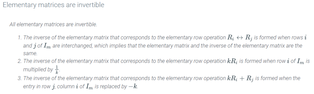
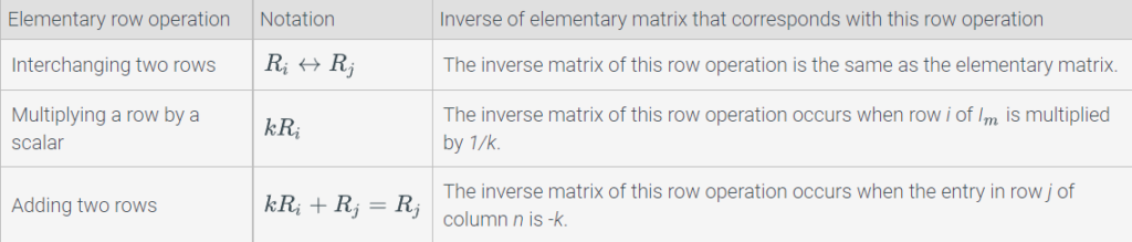
• All elementary matrices are invertible. The following summarizes their inverses

• A square matrix is invertible if and only if it is row equivalent to the identity matrix. That is, you could perform a sequence of elementary row operations to reduce the matrix to I.
• The invertible matrix theorem is an important theorem that identifies equivalent conditions on a square matrix. If A is a square matrix then the following are equivalent:
  • Matrix A is nonsingular.
  • Matrix A is not row equivalent to a matrix with a zero row or column.
  • The determinant of matrix A does not equal zero: det(A)≠0.
  • Matrix A can be expressed as a product of elementary matrices.
  • Matrix A is row equivalent to the identity matrix.

5.1 Unit 5: Finite and infinite series

The material in this unit comprises 10% of the high-stakes assessment and includes such concepts as:

• Geometric and arithmetic sequences
• Increasing, decreasing, and monotone sequences
• Infinite sequences
• Sum of finite and infinite series
• Convergence and divergence

If you deposit 500 dollars into the bank today and leave it there to earn 10% annual interest, how much will you have in 30 years?

• After the first year, you have: (OLD AMT) + 0.10(OLD AMT) = 500 + 0.10(500) dollars.
• After the second year, you have: (OLD AMT) + 0.10(OLD AMT) = [500 + 0.10(500)] + 0.10[500 + 0.10(500)] dollars.
• After the third year, you have: (OLD AMT) + 0.10(OLD AMT) = [500 + 0.10(500)] + 0.10[500 + 0.10(500)] + 0.10[500 + .10(500)] + 0.10[500 + 0.10(500)]] dollars.

5.2 Module 15: Overview of Sequences

• Introduction to sequences
• Increasing and decreasing sequences
• Geometric and arithmetic sequences

5.3 Lesson: Introduction to sequences

• After completing this lesson you should be able to find the value of the sequence at the specified term given an equation to define a finite sequence and a specified term (e.g., n = 8.)
• Sequences: Terms and notation
• Each element in a sequence is called a term. 
• Because there is a limited number of terms, this is a finite sequence.
• Sequences can also continue indefinitely. If we continue adding 2 to every term in the sequence from the example, we arrive to {2,4,6,8,10,12,14…}, which is an infinite sequence.
• Ellipses (…) are used to denote that there is no last element in an infinite sentence. The domain of an infinite sequence is the set of positive integers.
• The term an is called the nth term, or the general term, of the sequence.
• Finding terms in a sequence
• An explicit formula for a sequence allows you to find the value of any term in the sequence without determining all previous terms.
• Investigating piecewise explicit formulas

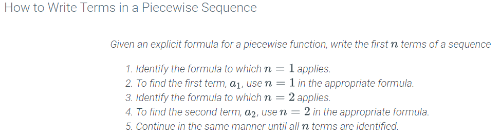
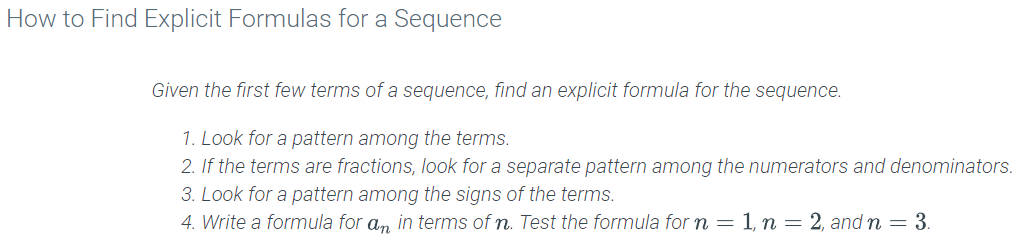
• Finding an explicit formula

• A sequence is an ordered set of objects, like numbers, that follow a particular pattern. The order is indicated by subscripts called indices. The numbers in the list are called terms of the sequence. The first term of sequence is called the initial term. If the sequence is finite, then the last term in the sequence is called, not surprisingly, the final term. The term is the nth term and often called the general term.
• An infinite sequence is a sequence with infinitely many terms. An infinite sequence has an initial term but not a final term. For example: a1,a2,a3,… (Ellipses are used to indicate the sequence goes on indefinitely.)
• If you can find a formula that generates the sequence then the sequence an=f(n) is explicitly defined. For example, an=3n+1,n≥1 generates the sequence: 4, 7, 10, …
• To find an explicit formula for a sequence, follow the steps:
  1. Look for a pattern among the terms
  2. If the terms are fractions, look for a pattern among denominators and look for a pattern among numerators
  3. Look for a pattern among the signs of the terms
  4. Write a conjecture for the general term an and test it for different values of n.
• A piecewise defined sequence is one that is defined differently for different groups of n. For example, it may be defined one way for even values of n and another for odd values of n.

5.4 Lesson: Increasing and decreasing sequences

• After completing this lesson you should be able to determine if a given finite sequence is increasing, decreasing, non‐decreasing, or non‐increasing.
• Increasing and decreasing sequences

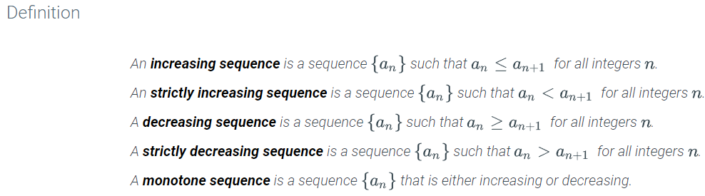
• A sequence {an} is eventually increasing if a positive integer n0 exists such that for all n>n0, an<an+1. For the sequence {cn}, n0=8. 

• A sequence is increasing if an<an+1 for all n and it is decreasing if an>an+1 for all n. For example: {1, 4, 9, 16, …} is an increasing sequence and {1, 1/2, 1/3, …} is a decreasing sequence.
• Sequences that are either only increasing or only decreasing are called monotone. Hint: The prefix “mono” means one, only, or single.
• A sequence can be neither increasing nor decreasing, and is therefore not monotone. For example, {2, 6, 1, 3, 2}.

5.5 Lesson: Geometric and arithmetic sequences

• After completing this lesson you should be able to find the value of the sequence at the specified term given an equation to define a geometric or arithmetic finite sequence and a specified term (e.g., n = 8).
• Geometric sequences
• A geometric sequence is a sequence that changes by a constant factor each year, as with the salary values described above. 4
• The constant factor by which a geometric sequences increases or decreases is called the common ratio.

• Writing terms of geometric sequences

• Using explicit formulas for geometric sequences

• Arithmetic sequences
• An arithmetic sequence is a sequence that changes by a constant amount for each term.
• Each term increases or decreases by the same constant value, which is called the common difference of the sequence. 

• Writing terms of arithmetic sequences

• Using explicit formulas for arithmetic sequences
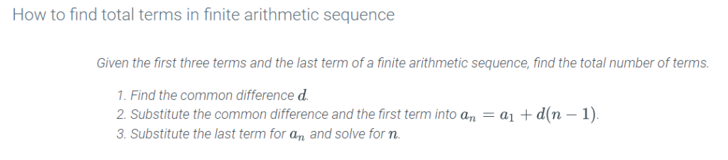
• Finding the number of terms in a finite arithmetic sequence

• A geometric sequence is of the form an=crn. The ratio of consecutive terms is the same (called the common ratio). For example, an=10×3n gives {30, 90, 270, 810,…} where the common ratio is: 9030=27090=810270=3
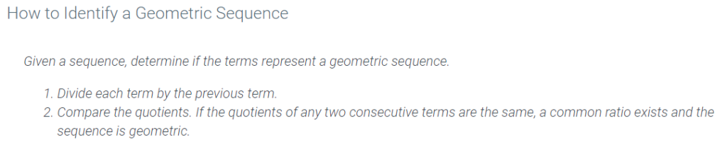
• To determine if a given sequence is geometric:
  1. Divide each term by the previous term
  2. Compare the quotients. If the quotients of every pair of consecutive terms is the same, then the sequence is geometric.
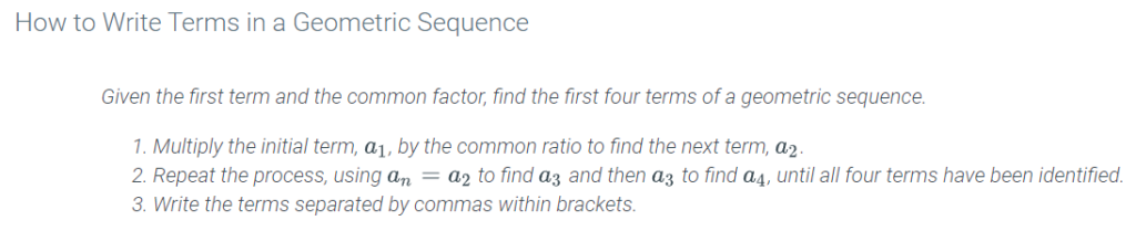
• To write terms in a geometric sequence with known initial term and common ratio:
  1. Multiply the initial term by the common ratio to find the second term
  2. Repeat the process to find the third term, and so on.
  3. Write the terms separated by commas within brackets.
• An arithmetic sequence is a sequence whose terms are of the form an=a1+(n−1)d. Consecutive terms are separated by the same distance (called the common difference).
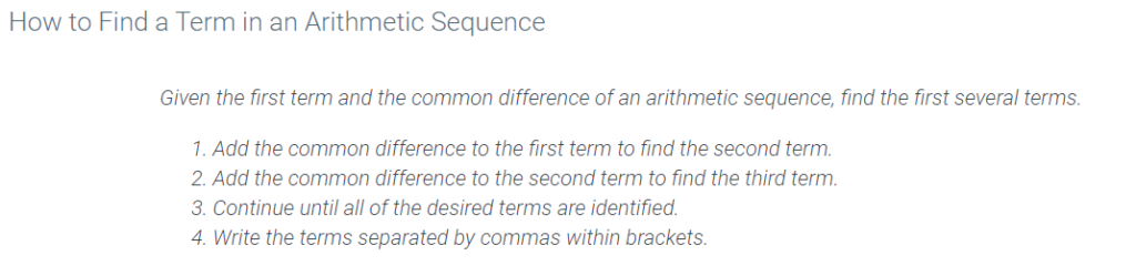
  {a1,a1+d,a1+2d,a1+3d,…}
• To find a term in an arithmetic sequence given the first term and common difference:
  1. Add the common difference to the first term to find the second.
  2. Add the common difference to the second to find the third, and so on.
  3. Write the terms separated by commas within brackets.
• To find the total number of terms in a finite arithmetic sequence given the first three terms and the last term:
  1. Find the common difference
  2. Plug into the formula the last term and the common difference for d and then solve for n in an=a1+(n−1)d.

5.6 Module 16: Sequences and Series

• Infinite sequences
• Sum of a finite series
• Sum of an infinite series
• Sequence: convergence and divergence
• Series: divergence test

5.7 Lesson: Infinite sequences

• After completing this lesson you should be able to solve for the formula of the general term of an infinite sequence.
• Limit of a sequence
• An infinite sequence{an} is an ordered list of numbers of the form a1,a2,…,an,…. The subscript n is called the index variable of the sequence. Each number an is a term of the sequence. Sometimes sequences are defined by explicit formulas, in which case an=f(n) for some function f(n) defined over the positive integers. In other cases, sequences are defined by using a recurrence relation. In a recurrence relation, one term (or more) of the sequence is given explicitly, and subsequent terms are defined in terms of earlier terms in the sequence.

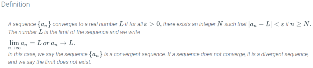
• Given a sequence {an}, if the terms an become arbitrarily close to a finite number L as n becomes sufficiently large, we say {an} is a convergent sequence and L is the limit of the sequence. In this case, we writelimn→∞an=L.

• If a sequence {an} is not convergent, we say it is a divergent sequence.

• An infinite sequence is an ordered list of infinitely many terms. An infinite sequence has an initial term but not a final term. For example: a1,a2,a3… (ellipses are used to indicate that the sequence goes on indefinitely). {an}n=1∞={an}=a1,a2,a3…
• If you can find a formula that generates the sequence then the sequence an=f(n) is explicitly defined. For example, an=3n+1,n≥1 generates the sequence: 4, 7, 10, …
• If terms in a sequence are defined in terms of previous terms, then the sequence is recurrently defined. For example: an=an−1+an−2 with a1=1,a2=3.

5.8 Lesson: Sum of a finite series

• In this lesson you will step back to finite sequences so you can explore how to find the sum of the terms of the sequence, which is referred to as a series. 
• After completing this lesson you should be able to calculate the sum of a finite sequence.
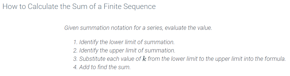
• Using summation notation
• The sum of the terms of a sequence is called a series.
• The nth partial sum of a sequence is the sum of a finite number of consecutive terms beginning with the first term.
• Summation notation is used to represent series, and is often known as sigma notation because of the use of the Greek capital letter sigma ∑ to represent the sum. 
• The index of summation is set equal to the lower limit of summation, the number used to generate the first term in the series. 
• The number above sigma is called the upper limit of summation, the number used to generate the last term in a series.

• Using the formula for arithmetic series

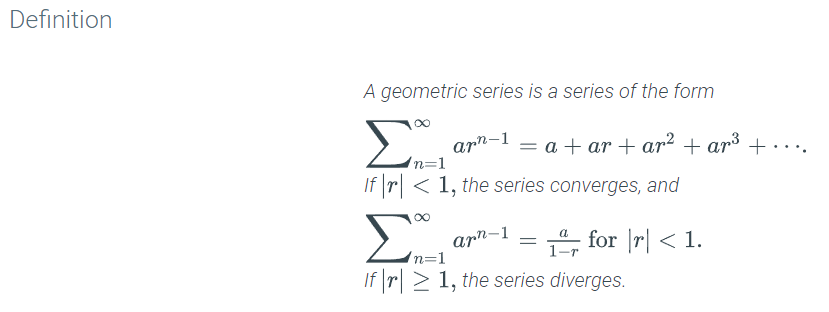
• Using the formula for geometric series

• A finite series is the sum of the finite number of terms in a finite sequence. The notation is: ∑n=1kan=a1+a2+…+ak
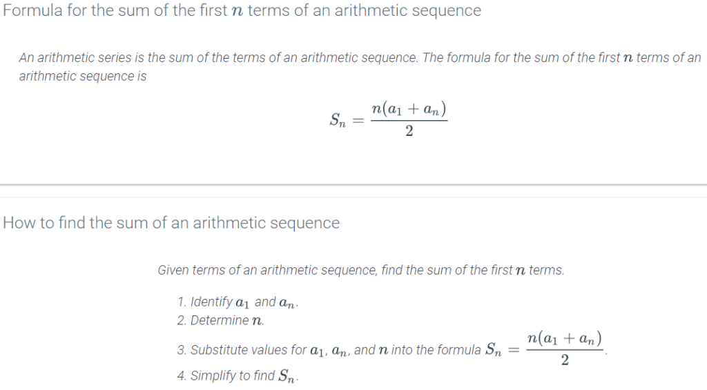
• The sum of a finite number of terms of an arithmetic sequence is Sn=∑k=1nan=n(a1+an)2.
• Use the following steps to find the sum of an arithmetic series:
  1. Identify a1,an
  2. Determine n
  3. Substitute values for a1,an and n into the formula Sn=n(a1+an)2
  4. Simplify the results
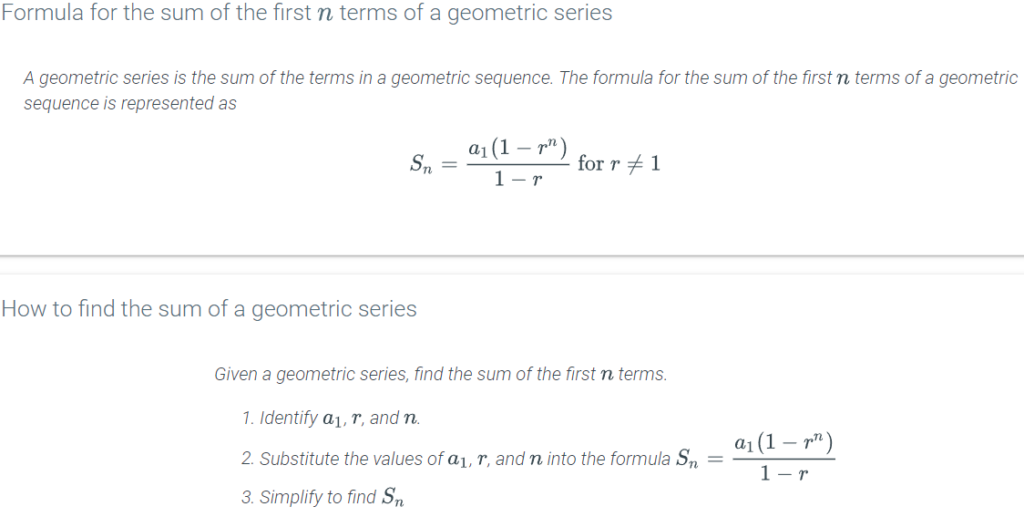
• The sum of a finite geometric sum is: Sn=∑k=0n−1ark=a(1−rn1−r)
• Use the following steps to find the sum of a geometric series:
  1. Identify a1,r,n
  2. Substitute values for a1,r and n into the formula Sn=a(1−rn1−r)
  3. Simplify the results

5.9 Lesson: Sum of an infinite series

• In this lesson you will learn how to determine if an infinite sequence series has a limit (converges) and how to calculate the sum using partial sums. 
• After completing this lesson you should be able to calculate the sum of an infinite geometric series using the limit of the sequence of partial sums.
• Sums and series
• An infinite series is an expression of the form ∑n=1∞an=a1+a2+a3+….
•  is called the kth partial sum of the infinite series.
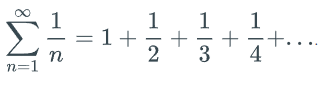
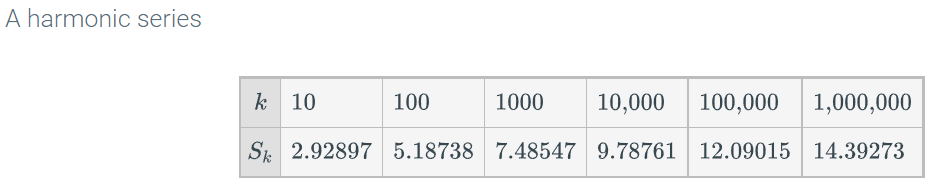
• The harmonic series
• The harmonic series is defined as

• Geometric series

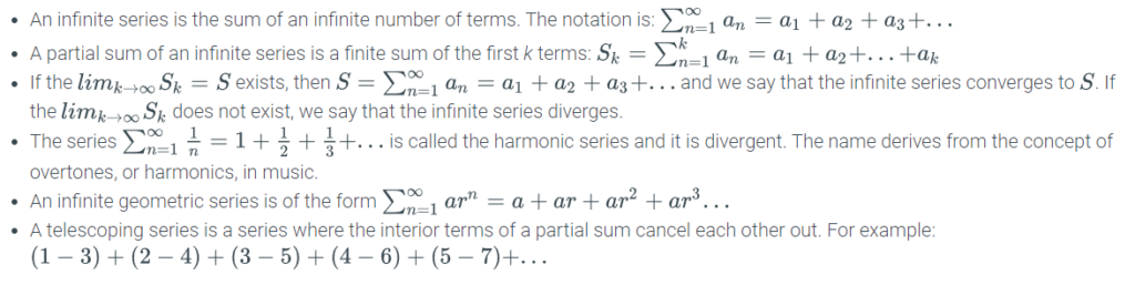
• Telescoping series

5.10 Lesson: Sequence convergence and divergence

• After completing this lesson you should be able to determine the limit of a given sequence if the sequence converges or if the sequence diverges.
• Convergence and divergence

• Algebraic Limit Laws

• Bounded sequences

• Informally, limn→∞an=L if an can be made arbitrarily close to L as n becomes sufficiently large.
• If the limit of a sequence exists, the sequence is said to converge to that limit. If the limit does not exist, the sequence is said to diverge.
• If a sequence is explicitly defined, an=f(n),n≥1 and if limx→∞f(x)=L, then {an} converges and we write limn→∞an=L.
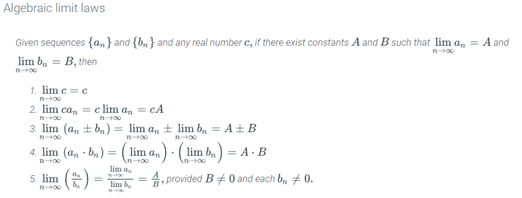
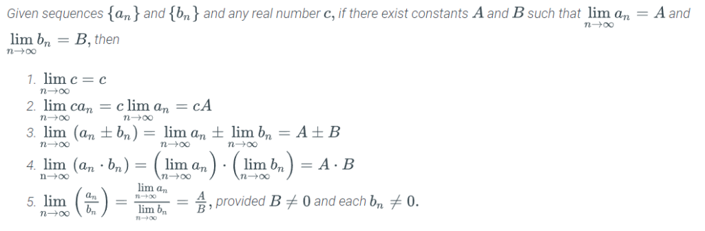
• Review the following algebraic limit laws:

5.11 Lesson: Series divergence test

• After completing this lesson you should be able to analyze the convergence or divergence of a series using the divergence test.
• Divergence test

• For a series ∑n=1∞an to converge, an→0 as n→∞.
• If limn→∞an≠0, then the series is said to diverge by the test for divergence.

6.1 Unit 6: Relations

• Binary relations, sets, and properties
• Binary relation properties and directed graphs
• Graph powers and matrix multiplication
• Partial order relations and Hasse diagrams
• Strict order relations
• N-ary relations

6.2 Module 17: Binary Relations and Directed Graphs

• Introduction to binary relations
• Binary relations: sets
• Binary relations: properties
• Binary relations: directed graphs

6.3 Lesson: Introduction to binary relations

• In this lesson you will use the information from those previous units to learn about a related concept: binary relations.
• After completing this lesson you should be able to evaluate the visual representations of binary relations.
• Binary relations
• Mathematically, a binary relation between two sets A and B is a subset R of A x B. 
• In an arrow diagram of a relation R on sets A and B, the elements of A are listed on the left, the elements of B are listed on the right, and there is an arrow from a ∈ A to b ∈ B if aRb.
• A matrix representation of relation R between A and B is a rectangular array of numbers with |A| rows and |B| columns.

• Binary Relation:
  • The binary relation, R, is a subset of the product of two sets. Given sets A and B, for a ∈ A and b ∈ B, (a, b) ∈ is denoted aRb.
  • For example, from your lessons on functions, Cartesian coordinates (ordered pairs) are considered binary relations of the domain, D, and range, R. The relationship, or function F, would be denoted in this section as dFr where d ∈ D and r ∈ R.
• Arrow Diagram: A binary relation, R, between two sets A and B, can be represented graphically using an arrow diagram.
  • Elements of set A are in the column on the left and elements of set B are in the column on the right. Arrows point from elements in set A to elements in set B as long as aRb. Note: This is very similar to the ordered pair lists in the previous chapter on functions.
• Matrix Representation: A matrix is a rectangular array of ones (1) and zeros (0). To represent the binary relation, R, between sets A and B in a matrix:
  • Create an array where the number of elements in A equals the number of rows and the number of elements in B equals the number of columns.
  • If aRb AND a ∈ A AND b ∈ B, put a “1” in the corresponding row/column. Otherwise, if the row/column combination is ∉ aRb, then put a “0” in that position.