Unit 1: Pre-Calculus Review

Unit 1 of Calculus I is optional review to prepare you to succeed in this course. It is provided only if you need it, but these concepts are foundational for building the skills and understandings covered in Units 2 through 5.

None of the material in this unit is specifically addressed in the final high-stakes assessment for Calculus I, other than as building blocks for the following units. This means you will need the skills in this unit to do everything in Units 2 through 5.

Note that there are few lesson introductions and no lesson exercises or summaries in these modules, unlike what you’ll see in the following units.

The modules in this unit are:

1. Review of parent functions
2. Graphs and equations of functions
3. Writing equations of lines
4. Average rates of change
5. Exponentials and graphs
6. Rules of exponents
7. Logarithms and graphs
8. Summation notation
9. Angles and radians
10. Sine and cosine
11. Other trigonometric functions
12. Trigonometric functions and graphs

Module A: Review of parent functions

This page is also the start of Module A. Please review this material if you need a stronger foundation in these concepts before beginning the central content for Calculus I in Unit 2.

1.2 Lesson: Graphs of parent functions

NOTE: The content in Unit 1, and in this specific lesson, is foundational for building the skills and understandings covered in the remainder of this learning resource, Units 2 through 5. However, since it is basically reference material, the content on this page will not be directly assessed on your high-stakes exam.

Lesson introduction

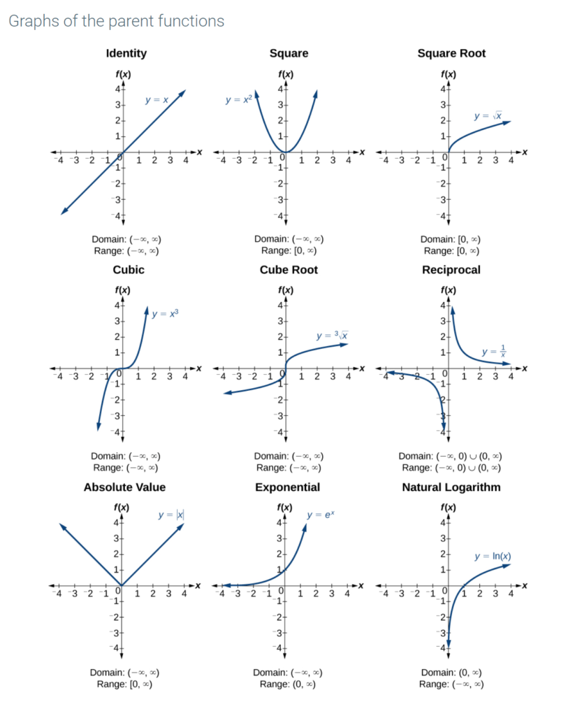
The nine graphs on this page are called “parent functions” because each one is the simplest form of a whole family of functions. The families are the identity functions, the square functions, the square root functions, the cubic functions, and so on.

Please become very familiar with these nine parent functions, as you will be seeing them many times in this course and in your career.

Graphs of parent functions

1.4 Lesson: Graphs and equations of functions

NOTE: The content in Unit 1, and in this specific lesson, is foundational for building the skills and understandings covered in the remainder of this learning resource, Units 2 through 5. However, since it is basically reference material, the content on this page will not be directly assessed on your high-stakes exam.

Lesson introduction

In just about any toolbox, you find a hammer, a saw, pliers, a wrench, and a screwdriver. These are our most basic hand tools, and simple as they are, you can actually do a lot with them. Similarly, we have a basic “toolkit” of nine functions, and we can do quite a lot with them, as well.

In this text, we will be exploring functions-the shapes of their graphs, their unique characteristics, their algebraic formulas, and how to solve problems with them. When learning to read, we start with the alphabet. When learning to do arithmetic, we start with numbers.

Identifying basic toolkit functions

When working with functions, it is similarly helpful to have a base set of building-block elements. We call these our “toolkit functions,” which form a set of basic named functions for which we know the graph, formula, and special properties. Some of these functions are programmed to individual buttons on many calculators. For these definitions we will use x as the input variable and y=f(x) as the output variable.

We will see these toolkit functions, combinations of toolkit functions, their graphs, and their transformations frequently throughout this book. It will be very helpful if we can recognize these toolkit functions and their features quickly by name, formula, graph, and basic table properties. The graphs and sample table values are included with each function shown in the figure below .

1.6 Lesson: Writing equations of lines

NOTE: The content in Unit 1, and in this specific lesson, is foundational for building the skills and understandings covered in the remainder of this learning resource, Units 2 through 5. However, since it is basically reference material, the content on this page will not be directly assessed on your high-stakes exam.

Lesson introduction

Just as with the growth of a bamboo plant, there are many situations that involve constant change over time. Consider, for example, the first commercial maglev train in the world, the Shanghai MagLev Train. It carries passengers comfortably for a 30-kilometer trip from the airport to the subway station in only eight minutes.^Note_Train

Suppose a maglev train were to travel a long distance, and that the train maintains a constant speed of 83 meters per second for a period of time once it is 250 meters from the station. How can we analyze the train’s distance from the station as a function of time? In this lesson, we will investigate a kind of function that is useful for this purpose, and use it to investigate real-world situations such as the train’s distance from the station at a given point in time.

Representing linear functions

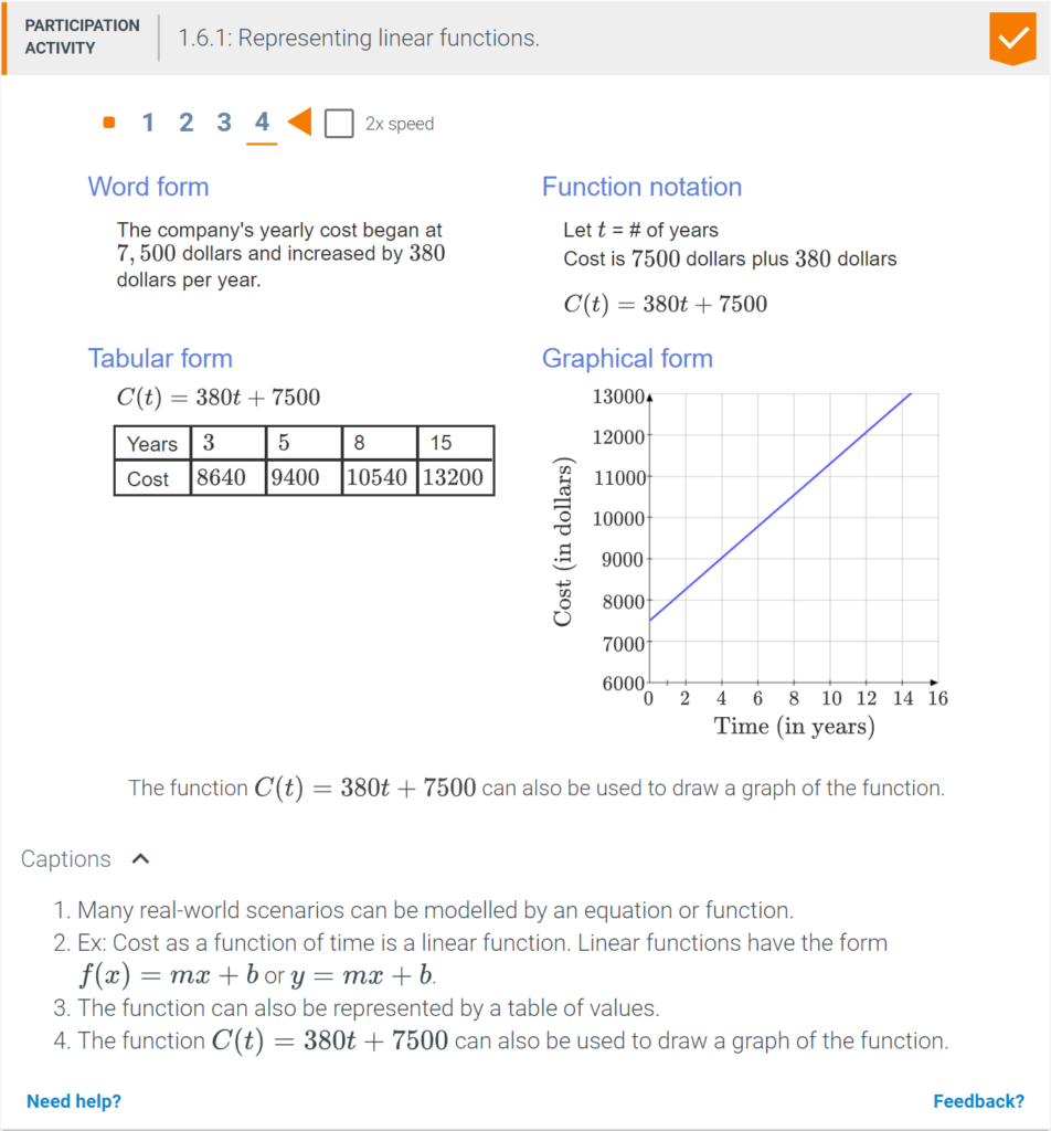
The function describing the train’s motion is a linear function, which is defined as a function with a constant rate of change, that is, a polynomial of degree 1. There are several ways to represent a linear function: (1) word form, (2) function notation, (3) tabular form, and (4) graphical form.

Representing a linear function in word form

Let’s begin by describing the linear function in words. For the train problem we just considered, the following word sentence may be used to describe the function relationship.

• The train’s distance from the station is a function of the time during which the train moves at a constant speed plus its original distance from the station when it began moving at constant speed.

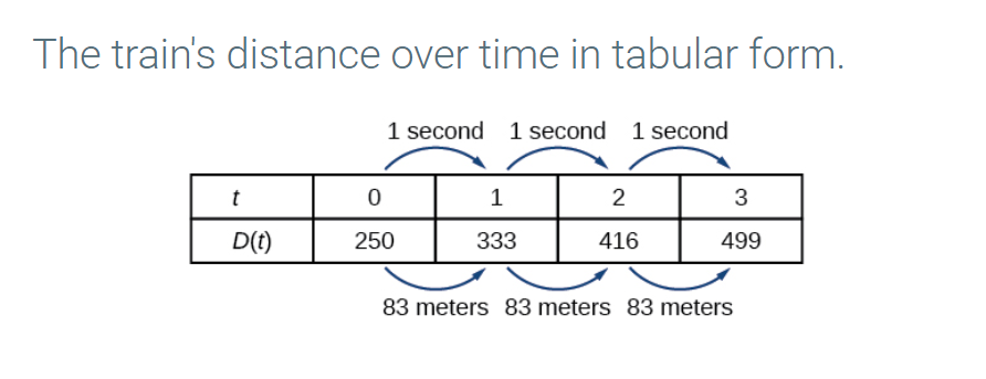
The speed is the rate of change. Recall that a rate of change is a measure of how quickly the dependent variable changes with respect to the independent variable. The rate of change for this example is constant, which means that it is the same for each input value. As the time (input) increases by 1 second, the corresponding distance (output) increases by 83 meters. The train began moving at this constant speed at a distance of 250 meters from the station.

Representing a linear function in function notation

Another approach to representing linear functions is by using function notation. One example of function notation is an equation written in the form known as the slope-intercept form of a line: f(x)=y=mx+b where x is the input value, m is the rate of change, and b is the initial value of the dependent variable.Equation formy=mx+bEquation notationf(x)=mx+b

In the example of the train, we might use the notation D(t) in which the total distance D is a function of the time t. The rate,m, is 83 meters per second. The initial value of the dependent variable b is the original distance from the station, 250 meters. We can write a generalized equation to represent the motion of the train.D(t)=83t+250

Representing a linear function in tabular form

A third method of representing a linear function is through the use of a table. The relationship between the train’s distance from the station and the time is represented in the table below. From the table, we can see that the distance changes by 83 meters for every 1 second increase in time.

Representing a linear function in graphical form

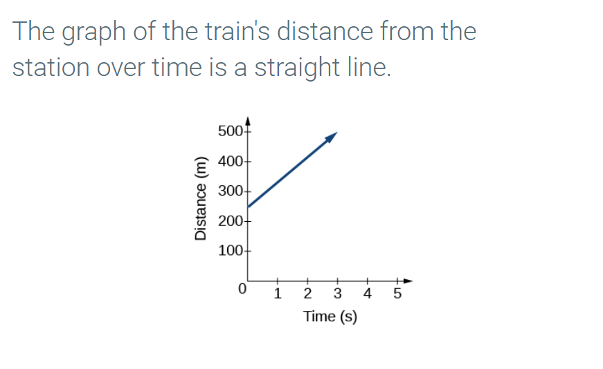
Another way to represent linear functions is visually, using a graph. We can use the function relationship from above, D(t)=83t+250, to draw a graph, represented in the figure below. Notice the graph is a line. When we plot a linear function, the graph is always a line.

The rate of change, which is constant, determines the slant, or slope of the line. The point at which the input value is zero is the vertical intercept, or y-intercept, of the line. We can see from the graph above that the y-intercept in the train example we just saw is (0,250) and represents the distance of the train from the station when it began moving at a constant speed.

Notice that the graph of the train example is restricted, but this is not always the case. Consider the graph of the line f(x)=2x+1 Ask yourself what numbers can be input to the function, that is, what is the domain of the function? The domain is comprised of all real numbers because any number may be doubled, and then have one added to the product.

Linear function

A linear function is a function whose graph is a line. Linear functions can be written in the slope-intercept form of a linef(x)=mx+b

where b is the initial or starting value of the function (when input, x=0 ). The rate of change of a linear function is called the slope, denoted by m. The y-intercept is at (0,b).

Determining whether a linear function Is increasing, decreasing, or constant

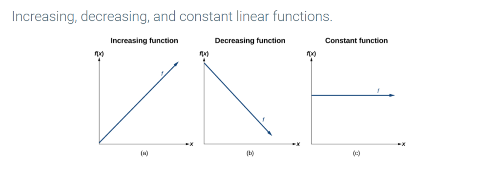
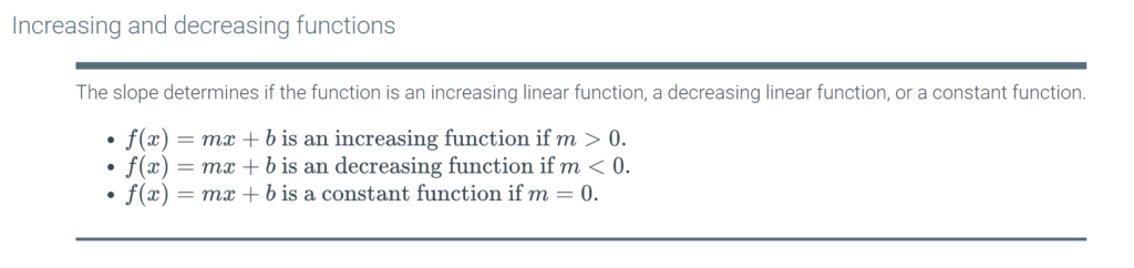
The linear functions we used in the two previous examples increased over time, but not every linear function does. A linear function may be increasing, decreasing, or constant. For an increasing function, as with the train example, the output values increase as the input values increase. The graph of an increasing function has a positive slope. A line with a positive slope slants upward from left to right as in the left graph (a) below. For a decreasing function, the slope is negative. The output values decrease as the input values increase. A line with a negative slope slants downward from left to right as in the middle graph (b) below. If the function is constant, the output values are the same for all input values so the slope is zero. A line with a slope of zero is horizontal as in the right graph (c) below.

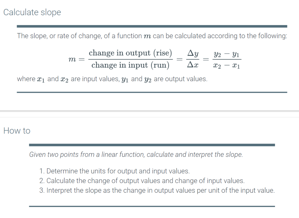
Calculating and interpreting slope

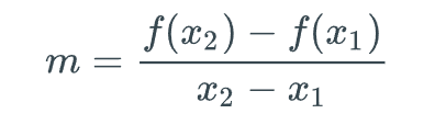
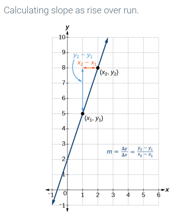
In the examples we have seen so far, we have had the slope provided for us. However, we often need to calculate the slope given input and output values. Given two values for the input,x1 and x2, and two corresponding values for the output, y1 and y2-which can be represented by a set of points, (x1,  y1) and (x2,  y2)-we can calculate the slope m, as follows

where Δy is the vertical displacement and Δx is the horizontal displacement. Note in function notation two corresponding values for the output y1 and y2 for the function f,y1=f(x1) and y2=f(x2), so we could equivalently write

The figure below indicates how the slope of the line between the points,(x1,y1) and (x2,y2), is calculated. Recall that the slope measures steepness. The greater the absolute value of the slope, the steeper the line is.

Question and answer

Are the units for slope always units for the outputunits for the input?

Yes. Think of the units as the change of output value for each unit of change in input value. An example of slope could be miles per hour or dollars per day. Notice the units appear as a ratio of units for the output per units for the input.

Writing the point-slope form of a linear equation

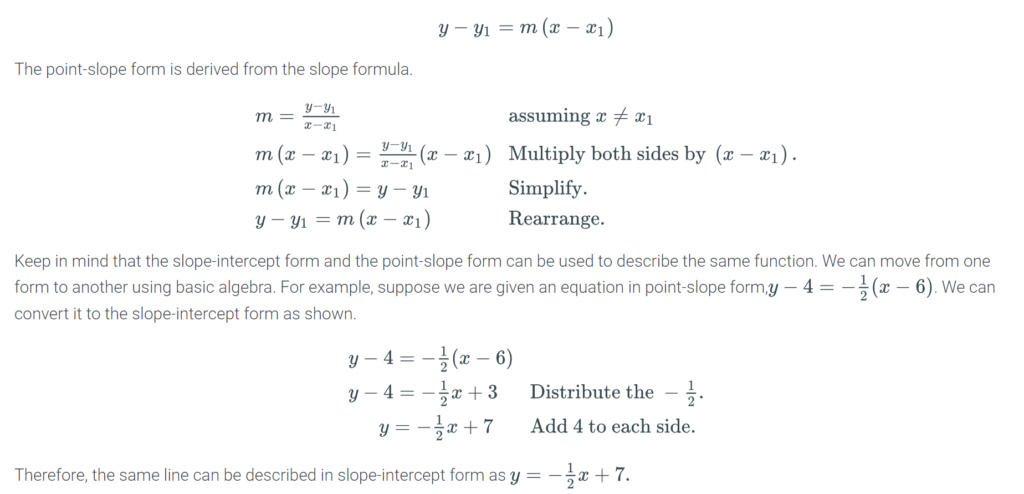
Up until now, we have been using the slope-intercept form of a linear equation to describe linear functions. Another way to write a linear function is called point-slope form, y−y1=m(x−x1) where m is the slope and (x1,y1) is any point on the line..

Lesson summary

Before moving on, take a last moment to think about what you’ve learned in this lesson:

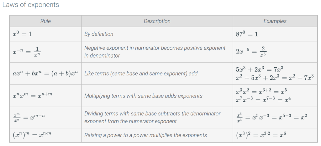
• Positive exponents indicate repeated multiplication (how many times something is multiplied by itself). Negative exponents indicate repeated division (or how many times you are dividing by a number – remember there’s always at least a “1” in the numerator). For example, x4=x⋅x⋅x⋅x and x−4=1x⋅x⋅x⋅x.
• When performing multiplication and division with exponents, there are several properties or short-cuts you can use to calculate the result. Make sure you know these properties/short-cuts to make working with exponents as efficient as possible.
• Zero raised to any non-zero power is equal to 0. Any non-zero number raised to the zero power is equal to 1. See this video for an argument why 00 is undefined.