7.4 Lesson: Graph theory and common graphs

• After completing this lesson you should be able to determine a graph’s properties (e.g., simple or multigraph, directed or undirected, cyclic or acyclic) and the vertex degree.
• Introduction to graph theory

• Undirected graphs in applications
• Molecular graphs: the vertices of the graph are the atoms in a molecule. There is an edge between two atoms if they form a bond. For molecular graphs, vertices are labeled with the type of atom they represent and edges are labeled with the type of bond they represent. The structure of a molecular graph reveals important information about the chemical properties of the molecule.
• Scheduling constraints: consider a school that has to schedule a set of courses for a given semester. The vertices of the graph represent the courses to be scheduled. There is an edge between two vertices if the corresponding courses have a conflict. For example, if the meeting times of the courses have already been determined, two courses that have overlapping times can not be scheduled in the same room. There would be an edge between any two courses whose meeting times overlap.
• Communication network: the vertices of a graph denote switches in a communication network. There is an edge between two switches if there is a two-way communication link between the two switches. Network designers would like to design a communication network such that even if a few communication links fail, it is still possible for every switch in the network to send a message to every other switch.
• Social network: consider a graph whose vertices represent individuals. There is an edge between two people if they are acquainted. (Assume that the property of being acquainted is mutual: if person A is acquainted with with person B, then person B is acquainted with person A). Sociologists study social networks to understand how information spreads in communities or how societies evolve. The advent of online social networks has allowed social scientists to study social patterns on a much larger scale.
• Common graphs

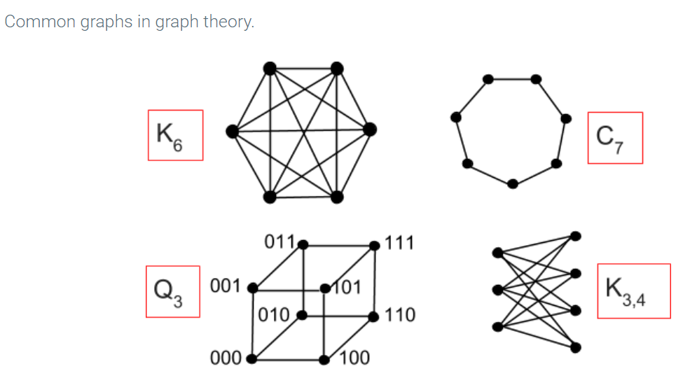
• K_n is called the complete graph on n vertices. K_n has an edge between every pair of vertices. The figure shows K₆. K_n is sometimes called a clique of size n or an n-clique.
• In an undirected graph, the total degree of the graph G is 2 times the number of edges in G. This can be shown through mathematical induction, which is a common proof technique used in graph theory.
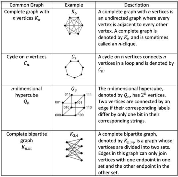
• Review the characteristics and names of common undirected graphs:

7.5 Lesson: Undirected graph representations

• After completing this lesson you should be able to determine if two undirected graphs are equivalent using either the adjacency list or the matrix representation of the graph.
• Adjacency list representation for graphs
• In the adjacency list representation of a graph, each vertex has a list of all its neighbors.
• Matrix representation for graphs
• The matrix representation for a graph with n vertices is an n by n matrix whose entries are all either 0 or 1, indicating whether or not each edge is present. 

• Undirected graphs with the same set of vertices and edges are the same graph even though their drawings may look different.
• To input data modeled by a graph into a computer program, there needs to be a formal way to represent the graph that the computer can interpret. There are two graph representations: adjacency list and matrix representation.
• An adjacency list representation is a graph representation which includes a list of all vertices and their neighbors (vertices connected by an edge).
• A matrix representation of a graph consists of a (n × n) matrix M whose columns and rows correspond to the vertices of the graph.
  • A cell in the matrix M is denoted Mi,j where the row corresponds to the vertex i and the column corresponds to the vertex j.
  • A 1 is placed in a cell if there is an edge connecting the vertices that correspond to the column and row of the cell. Mi,j = 1 if {i,j} is an edge in the graph
  • A 0 is placed in the cell if there is no edge connecting the corresponding vertices. Mi,j =0 if {i,j} is not an edge in the graph.
• Both the adjacency list representation and the matrix representation will help you to determine the complexity of the graph and, in turn, the time it will take the computer to interpret its data.

7.6 Lesson: Graph isomorphism

• After completing this lesson you should be able to identify the graph properties preserved under isomorphism.
• Graph isomorphism
•  Two graphs are said to be isomorphic if there is a correspondence between the vertex sets of each graph such that there is an edge between two vertices of one graph if and only if there is an edge between the corresponding vertices of the second graph. 
• Let G = (V, E) and G’=(V’,E’). G and G’ are isomorphic if there is a bijection f: V → V’ such that for every pair of vertices x, y ∈ V, {x, y} ∈ E if and only if {f(x), f(y)} ∈ E’. The function f is called an isomorphism from G to G’.
• A property is said to be preserved under isomorphism if whenever two graphs are isomorphic, one graph has the property if and only if the other graph also has the property. 
• The degree sequence of a graph is a list of the degrees of all of the vertices in non-increasing order. 
• The number and degree of vertices, number of edges, and degree sequence are structural properties of graphs.
• If the structural properties of two graphs are the same they are isomorphic. Let G = (V, E) and G’=(V’,E’). G and G’ are isomorphic if there is a bijection f: V → V’ such that for every pair of vertices x, y ∈ V, {x, y} ∈ E if and only if {f(x), f(y)} ∈ E’. The function f is called an isomorphism from G to G’.
• If two graphs have either a different number of edges or a different number of vertices, they are not isomorphic.
• Structural properties of two isomorphic graphs that remain the same for every isomorphism defined between them are called properties preserved under isomorphism.
• The degree of vertex v in graph G is the same as the degree of f(v) in G’ if f is an isomorphism between G and G’. That is, the degree of a vertex is a property preserved under isomorphism for every vertex v.
• Listing the degrees of each vertex of a graph G from largest to smallest is called the degree sequence of a graph. The degree sequence is a property preserved under isomorphism.
• You can determine that graphs are not isomorphic by examining properties that are preserved under isomorphism. If two graphs differ on any of these properties, they are not isomorphic.
• The labeling of the vertices is not a property preserved under isomorphism, so two graphs can be isomorphic even if the vertices have different labels.

7.7 Module 22: Paths, Circuits, and Cycles

• Paths, cycles, and connectivity
• Graph connectivity

7.8 Lesson: Paths, cycles, and connectivity

• After completing this lesson you should be able to solve for the longest path, circuit, or cycle with n vertices in an undirected graph.
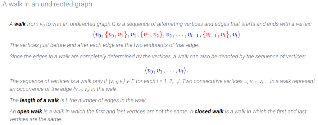
• A walk from v₀ to v_l in an undirected graph G is a sequence of alternating vertices and edges that starts and ends with a vertex:
• The length of a walk is l, the number of edges in the walk.
• An open walk is a walk in which the first and last vertices are not the same. A closed walk is a walk in which the first and last vertices are the same.

• A trail is an open walk in which no edge occurs more than once.
• A circuit is a closed walk in which no edge occurs more than once.
• A path is a trail in which no vertex occurs more than once.
• A cycle is a circuit of length at least 1 in which no vertex occurs more than once, except the first and last vertices which are the same.

• A sequence of alternating vertices and edges that begin and end with a vertex is called a walk. You can denote the walk as a sequenced list of vertices with the understanding that there is an edge connecting adjacent vertices. For example, in the sequence below the walk begins with vertex v0 and ends with vertex vl .⟨v0,v1,…,vl⟩.
• The number of edges is referred to as the length of the walk. In the above example, the length of the walk is l.
• A walk where no vertex is repeated is called a path.
• If there exists a walk between vertex a and vertex b in a graph G, then there also exists a path in G that begins with vertex a and ends with vertex b.
• If the first vertex is the same as the last vertex, the walk is called a circuit. For example, <a,b,c,b,a>. If the circuit is at least three lengths and contains no repeated vertex other than the beginning and end, it is called a cycle. For example, <a,b,c,d,a>.
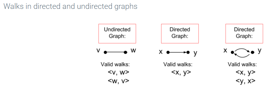
• If <v,w,x,s> is a walk in an undirected graph, then so is <s,x,w,v> because the edges have no defined direction. If <v,w,x,s> is a walk in a directed graph, <s,x,w,v> is not necessarily a walk.

7.9 Lesson: Graph connectivity

• After completing this lesson you should be able to determine the connectivity of an undirected graph using either the edges or the vertices, including k‐edge‐connectivity or k‐vertex‐ connectivity.
• Connected components
• In an undirected graph, if there is a path from vertex v to vertex w, then there is also a path from w to v. The two vertices, v and w, are said to be connected. 
• A graph is said to be connected if every pair of vertices in the graph is connected, and is disconnected otherwise.
• k-connectivity
• k-vertex-connected graph

• An undirected graph G is k-vertex-connected if the graph remains connected after any k – 1 vertices are removed from the graph. The vertex connectivity of a graph is the largest k such that the graph is k-vertex-connected. The vertex connectivity of a graph G is denoted κ(G).

• The vertex connectivity of a graph is the minimum number of vertices whose removal disconnects the graph into more than one connected component.
• k-edge-connected graph

• An undirected graph G is k-edge-connected if it remains connected after any k – 1 edges are removed from the graph. The edge connectivity of a graph is the largest k such that the graph is k-edge-connected. The edge connectivity of a graph G is denoted λ(G).

• The edge connectivity of a graph is the minimum number of edges whose removal disconnects the graph into more than one connected component.

• A set of vertices in a graph is connected if there is a path between every pair of vertices in that set.
• A graph is connected if its entire vertex set is connected, otherwise it is disconnected.
• If a graph is disconnected it can be divided into its connected pieces called components. A component is a maximally connected set of vertices, meaning that if an additional vertex is added from the set of all the vertices in G, the collection will no longer be connected.
• An isolated vertex is one that is not connected to any other vertex.
• An undirected graph G is k-vertex- connected if the graph remains connected after any k – 1 vertices are removed from the graph. For example, a graph is 4-vertex- connected if it is still connected after removing 3 vertices from the graph.
• The vertex connectivity of the graph, denoted κ(G), is the largest k such that the graph is k-vertex- connected. For example, if a graph is 5-vertex- connected (but not 6) then it is also 4-vertex- connected, and 3-vertex- connected and so on. However, the vertex connectivity of the graph is κ(G)=5.
• Similar definitions exist for edges where λ(G) represents the edge connectivity.
• κ(G)≤δ(G) and λ(G)≤δ(G) where δ(G) is the minimum degree of any vertex in G.
• Graph connectivity is an equivalence relation.

7.10 Module 23: Paths and Cycles in Trees

• Introduction to trees
• Properties of trees

7.11 Lesson: Introduction to trees

• After completing this lesson you should be able to determine the elements of an undirected tree graph including parents, ancestors, children, leaves, siblings, and subtrees.
• File system on a computer

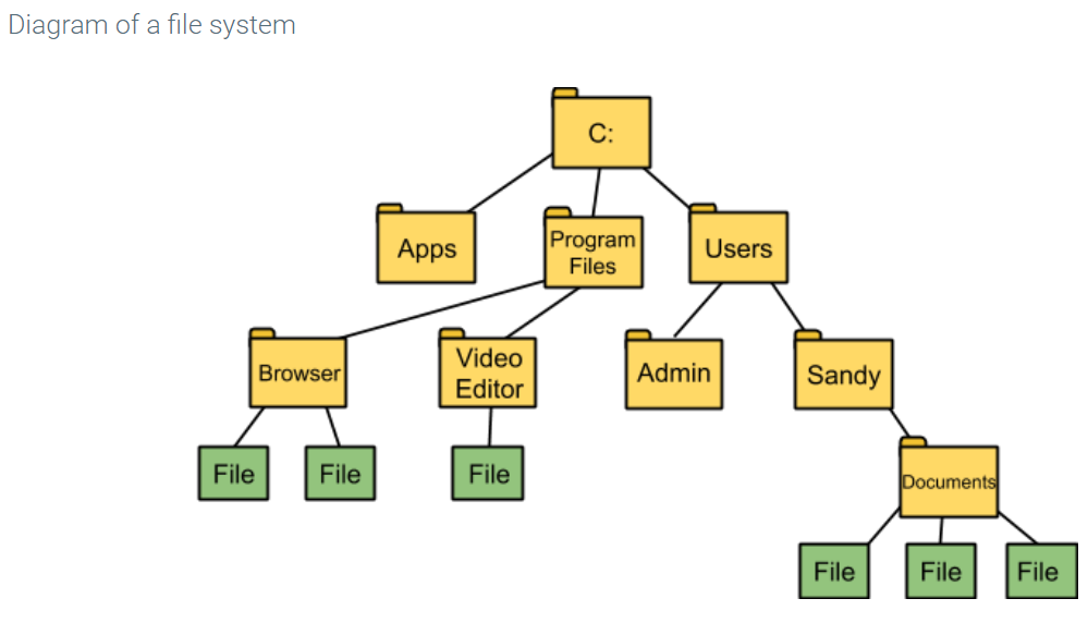
• A tree is an undirected graph that is connected and has no cycles.

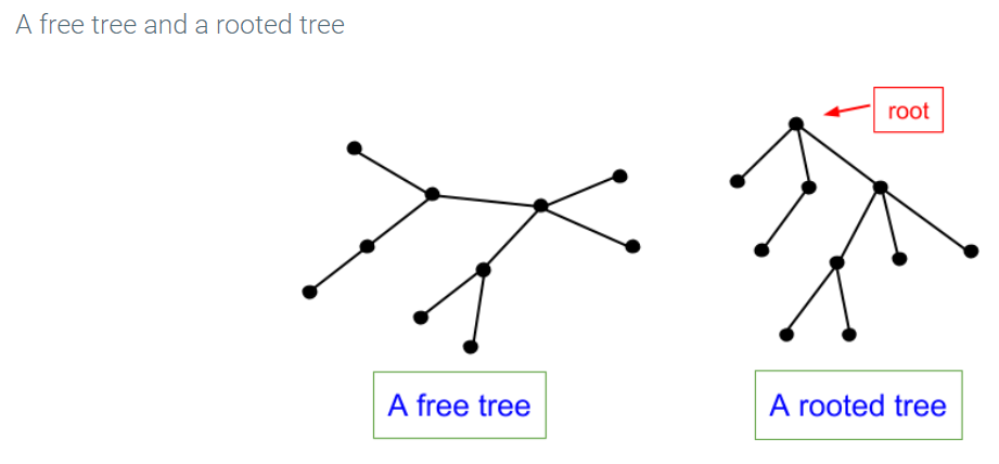
• The tree on the left is called a free tree because there is no particular organization of the vertices and edges.
•  The tree on the right is called a rooted tree.
• The vertex at the top of the drawing is designated as the root of the tree. 
• The level of a vertex is its distance from to the root. 
• The height of a tree is the highest level of any vertex. The tree on the right has height 3.
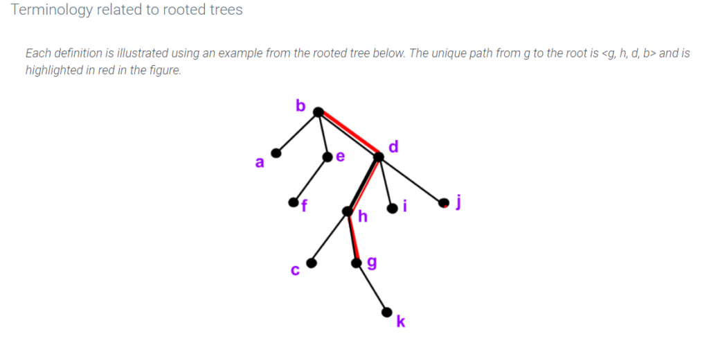
• Every vertex in a rooted tree T has a unique parent, except for the root which does not have a parent. The parent of vertex v is the first vertex after v encountered along the path from v to the root. (Ex: The parent of vertex g is h.)
• Every vertex along the path from v to the root (except for the vertex v itself) is an ancestor of vertex v. (Ex: The ancestors of vertex g are h, d, and b.)
• If v is the parent of vertex u, then u is a child of vertex v. (Ex: Vertices c and g are the children of vertex h.)
• If u is an ancestor of v, then v is a descendant of u. (Ex: The descendants of vertex h are c, g, and k.)
• A leaf is a vertex which has no children. (Ex: The leaves are a, f, c, k, i, and j.)
• Two vertices are siblings if they have the same parent. (Ex: Vertices h, i, and j are siblings because they have the same parent, which is vertex d.)
• A subtree rooted at vertex v is the tree consisting of v and all v’s descendants. (Ex: The subtree rooted at h includes h, c, g, and k and the edges between them.)

• A connected, undirected graph that contains no cycles is called a tree.
• A tree drawn with no particular organization of the vertices is called a free tree. A tree that appears to grow from a single vertex, the root, is called a rooted tree. The distinction is only in the intentional drawings of the tree.
• The level of a vertex is its distance away from the root. Distance is measured by the number of edges of the shortest path between the vertices. The height of the tree is the highest level of a vertex. That is, the height is the greatest distance any vertex is away from the root.
• Given any two vertices in a tree, there is only one path between them. In particular, every vertex in a rooted tree has only one path to the root.
• Every vertex in a rooted tree has only one path to the root.
• Some important definitions:The parent of a vertex v is the first vertex encountered on a path from v to the root.
• Every vertex in the path from v to the root is called an ancestor. The parent is the first encountered ancestor on the path.
• If u is the parent of v, then v is a child of u.
• If u is an ancestor of v, then v is a descendent of u.
• Vertices with no children are called leaves.
• Vertices with the same parent are called siblings.
• A subtree rooted at vertex v is the tree consisting of v and all v‘s descendants.

7.12 Lesson: Properties of trees

• After completing this lesson you should be able to analyze the paths, cycles, and properties of a tree graph.
• Theorem of unique paths in a free and rooted tree
•  A leaf of a free tree is a vertex of degree 1.
• A vertex is an internal vertex if the vertex has degree at least two

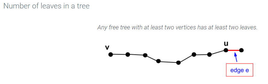
• Remember, in a rooted tree a vertex without children is called a leaf.
  • In a free tree with more than one vertex, a leaf is a vertex of degree 1.
  • In a free tree with only one vertex, the vertex has degree 0 but is still considered a leaf.
• In a free tree, vertices with a degree of at least 2 are called internal vertices.
• Any free tree with at least two vertices has at least two leaves.
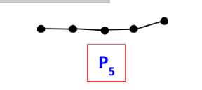
• Pn is a type of graph that consists of only a path with n vertices.

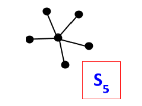
Sn is called a star graph. It consists of a vertex connected to n vertices by a single edge.

• A forest is a graph that consists of a collection of trees.
• A forest with c components and n vertices has n – c edges where n ≥ c.
• If G is an undirected graph with n vertices and m edges and if m < n – 1, then G is not connected.

7.13 Module 24: Tree Traversals and Spanning Trees

• Tree traversals
• Spanning trees: breadth-first and depth-first search
• Minimum spanning trees

7.14 Lesson: Tree traversals

• After completing this lesson you should be able to solve for post‐order and pre‐order traversals in a tree diagram.
• Tree traversal
• A common procedure performed on a tree (called a tree traversal) is to process the information stored in the vertices by systematically visiting each vertex.

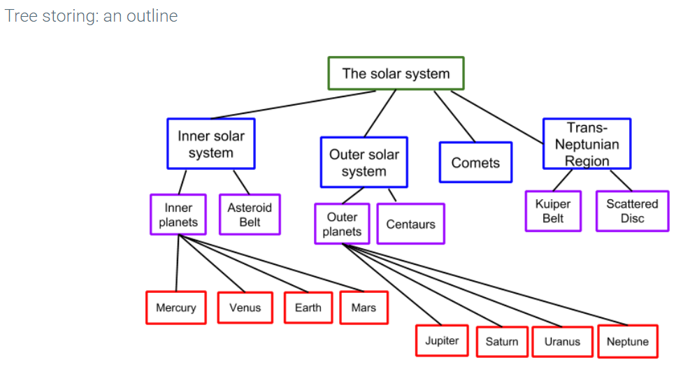
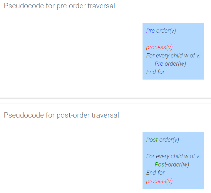
• In a pre-order traversal, a vertex is visited before its descendants. 

• Post-order traversal
• Scanning every vertex in a tree is called a tree traversal.
• A tree traversal that visits a vertex BEFORE its descendants is called a pre-order traversal.
• A tree traversal that visits a vertex AFTER its descendants is called a post-order traversal.
• The tree traversal algorithms are how the computer reads the data encoded in the tree.
• The post-order traversal is useful to count the number of leaves in a tree.

7.15 Lesson: Spanning trees- Breadth-first and depth-first search

• After completing this lesson you should be able to find spanning trees in a graph using breadth‐first search and depth‐first search.
• Spanning trees
• A spanning tree of a connected graph G is a subgraph of G which contains all the vertices in G and is a tree.

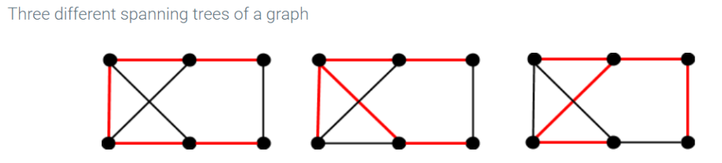
• There are two common methods for finding spanning trees in a graph: Breadth-First Search and Depth-First Search.
• Graph traversal is a process that systematically explores all the vertices of a graph. 
• Depth-First Search

• Breadth-first-search
• A subgraph of a connected graph is a spanning tree if it is a tree that contains all of the vertices of G.
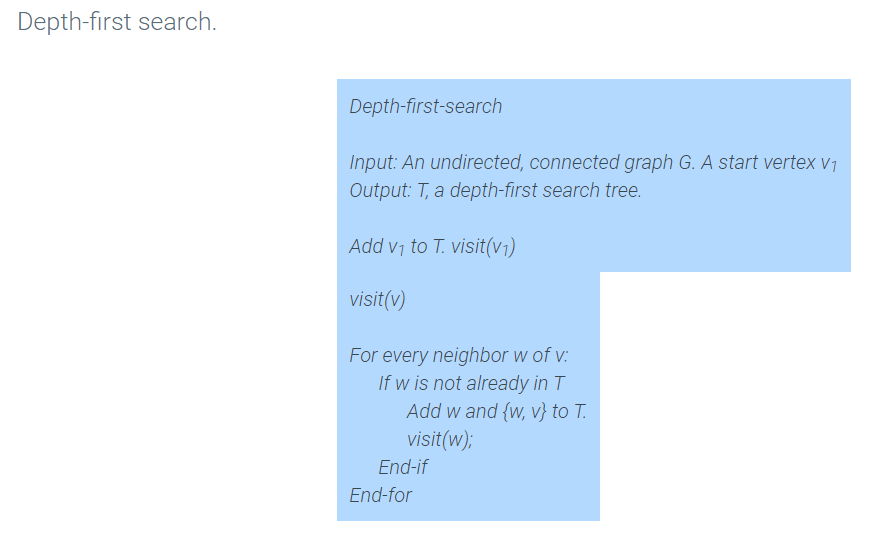
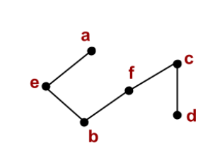
• In the depth-first search, starting at a root vertex, scan each neighbor and its neighbors and their neighbors. Once a neighbor has no more neighbors, back track to the previous neighbor and exhaust its neighbors. For example, if b and c are both neighbors of the root a, scan b and all its neighbors before backtracking to scan the neighbors of c.
• In the graph below, let a be the root vertex.

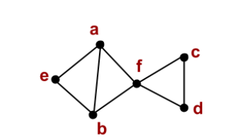
• Pick one of the neighbors of a-for example, e-and add the edge {a,e}.
• Pick a neighbor of e that has not already been scanned-for example, b-and add edge {e,b}.
• Pick a neighbor of b that has not already been scanned, say f, and add the edge {b,f}.
• Pick a neighbor of f that has not already been scanned, say c, and add the edge {f,c}.
• Pick a neighbor of c that has not already been scanned, say d, and add the edge {c,d}.

• In breadth-first search, starting at a root vertex scan each neighbor before scanning their neighbors. For example, if b and c are neighbors of the root a, scan b and c before scanning the neighbors of b.
• In the graph below, let a be the root vertex.
  

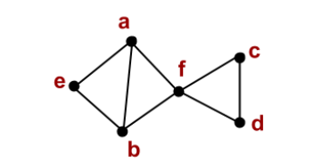
• Add the edges {a,e}, {a,b}, and {a,f}.
• Find the neighbors of e. The only neighbors of e are a and b, which are already included, so go to the next vertex, b.
• Find the neighbors of b. Since the only neighbors of b are e, a, and f, which are already included, go to the next vertex, f.
• Find the neighbors of f. The neighbors of f are c and d, both of which have not been added. Add the edges {f,c} and {f,d}.
• Repeat this procedure on c and d. Since the neighbors of the vertices c and d have been added, you have completed the search.

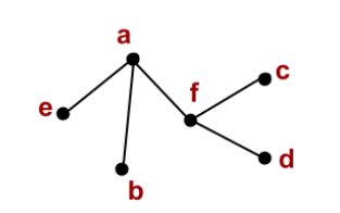
• A breadth-first search tree is likely the preferred spanning tree when you are looking for the shortest paths from the initial (source) vertex.
• An edge e belongs to every spanning tree if and only if removing e from the graph disconnects the graph into one or more connected components.

7.16 Lesson: Minimum spanning trees

• After completing this lesson you should be able to find the minimum weight spanning tree for a weighted graph.
• Spanning tree of a graph
• A weighted graph is a graph G = (V ,E), along with a function w: E → R. The function w assigns a real number to every edge.

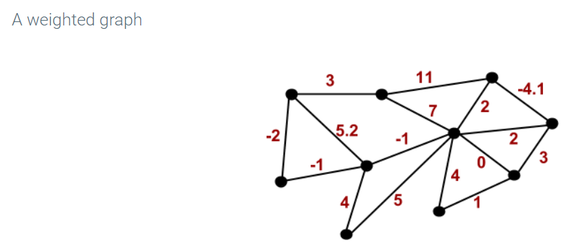
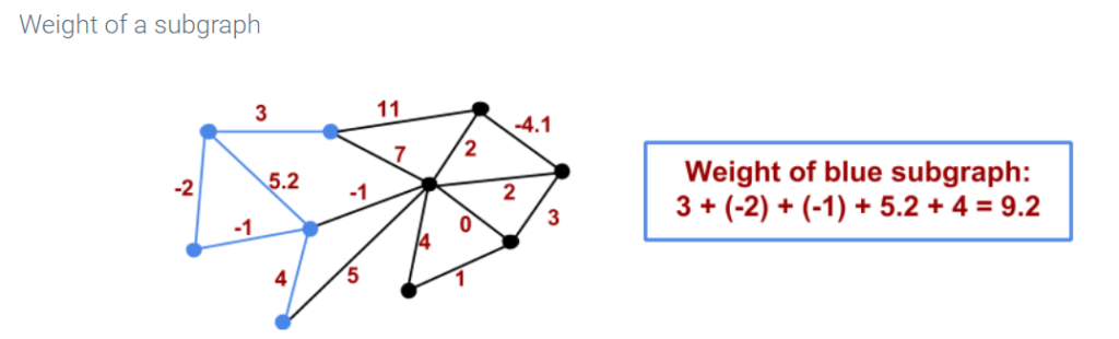
• A minimum spanning tree (MST) of a weighted graph, is a spanning tree T of G whose weight is no larger than any other spanning tree of G.
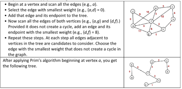
• Prim’s algorithm for minimum spanning tree
• Prim’s algorithm for finding and MST.

Input: An undirected, connected, weighted graph G.
Output: T, a minimum spanning tree for G.

T := ∅.
Pick any vertex in G and add it to T.

For j = 1 to n-1
      Let C be the set of edges with one endpoint inside T and one endpoint outside T.
      Let e be a minimum weight edge in C.
      Add e to T.
      Add the endpoint of e not already in T to T.
End-for

• Prim’s Algorithm : Prim’s algorithm finds a minimum spanning tree of the input weighted graph.

• All spanning trees with n vertices has n – 1 edges.
• A weighted graph is a graph G = (V, E), along with a function w: E → R. The function w assigns a real number to every edge. That is, each edge has assigned to it some value called a weight.
• The weight of a graph, or a subgraph, is the sum of the weights for each edge.
• A minimum spanning tree (MST) of a weighted graph, is a spanning tree T of G whose weight is no larger than any other spanning tree of G.
• An MST is not necessarily unique. That is, there can be more than one minimum spanning tree in a graph.
• A classic algorithm for finding a minimum spanning tree is Prim’s algorithm. The following is an example of how to apply Prim’s algorithm.