8 pages

2.1 Relational model

Database models

A database model is a conceptual framework for database software.

Leading database models of the 1960s, such as the hierarchic and network models, optimized processing speed at the expense of programmer productivity. As computer speed increased and programs became more complex, programmer productivity became paramount. A simpler approach was needed.

E. F. Codd created the relational model in the 1970s in response to the complexity of existing databases. The model was first implemented as System R at IBM in the late 1970s then released as DB2 in the early 1980s. Oracle and other relational databases were released around the same time.

The simplicity of relational databases was apparent to computer professionals. However, early product versions were slow compared to established databases. As relational processing speed caught up in the 1980s, relational products rapidly dominated the database market.

The advent of the internet in the 1990s generated massive volumes of online data, called big data, often with poorly structured or missing information. The relational model is not optimized for big data. As a result, many non-relational databases have come to market since 2000, optimized for big data and collectively called NoSQL databases. NoSQL stands for ‘Not only SQL’ and encompasses a variety of database models. NoSQL models and databases are described elsewhere in this material.

Despite the proliferation of NoSQL databases, relational remains the dominant model. Relational databases dominate applications that require an accurate record of every transaction, such as banking, airline reservation systems, and student records.

Table 2.1.1: Example database models.

Model	Inventor	Initial releases	Objectives	Example databases
Hierarchical	IBM	1960s	Speed and storage	IMS
Network	Charles Bachman	1960s	Speed and storage	IDMS
Relational	E. F. Codd	1980s	Productivity and simplicity Transactional applications	MySQL Oracle SQL Server DB2
NoSQL models	Google Amazon and others	2000s	Big data Analytic applications	MongoDB Redis Cassandra Neo4j

Relational data structure

The relational model is a database model based on mathematical principles, with three parts:

1. A data structure that prescribes how data is organized.
2. Operations that manipulate data structures.
3. Rules that govern valid relational data.

The relational data structure and operations are based on set theory. A set is a collection of values, or elements, with no inherent order. Sets are denoted with braces. Ex: {apple, banana, lemon} is the set containing three kinds of fruit. Since sets have no order, {apple, banana, lemon} is the same set as {lemon, banana, apple}.

The relational data structure is based on three mathematical concepts:

• A domain is a named set of possible database values, such as integers, dictionary words, or logical values TRUE and FALSE.
• A tuple is a finite sequence of values, each drawn from a fixed domain. Ex: (3, apple, TRUE) is a tuple drawn from domains (Integers, DictionaryWords, LogicalValues).
• A relation is a named set of tuples, all drawn from the same sequence of domains. Ex: The relation below is named Grocery and contains three tuples.

Since a relation is a set, the relation tuples have no inherent order.

Each tuple position is called an attribute. Each attribute has a name that is unique within the relation. Since each tuple position has a domain, each attribute also has a domain. Ex: In the Grocery relation, the first, second, and third positions might be named Quantity, FruitType, and OrganicCertification, with domains Integers, DictionaryWords, and LogicalValues, respectively.

Domain, tuple, relation, and attribute are mathematical terms. Data type, row, table, and column are equivalent terms, commonly used in database processing. This material uses the common database terms.

Table 2.1.2: Equivalent relational terms.

Mathematical	Database	Files
Domain	Data type	Data type
Tuple	Row	Record
Relation	Table	File
Attribute	Column	Field

Terminology

Relational tuples differ from mathematical tuples in one respect. In mathematics, the order of tuple values is significant. Ex: The tuples (7, 2) and (2, 7) are different. In the relational model, the order of tuple values is not significant, since each value is associated with a different attribute name.

Relational operations

The relational model stipulates a set of operations on tables, collectively called relational algebra. Like the relational data structure, relational operations are based on set theory. Relational operations include:

• Select — selects a subset of rows of a table.
• Project — eliminates one or more columns of a table.
• Product — lists all possible combinations of rows of two tables.
• Join — a product operation followed by a select operation.
• Union — combines two tables by selecting all rows of both tables.
• Intersect — combines two tables by selecting only rows common to both tables.
• Difference — combines two tables by selecting rows that appear in one table but not the other.

Relational algebra is the theoretical foundation of the SQL language.

The result of relational operations is always a table. Similarly, the result of a SQL statement is always a table. Although result tables are not stored in the database, result tables have the same data structure as stored tables.

Understanding the mathematics of these operations is interesting but not necessary. Understanding the corresponding SQL statements is more practical and useful for database programming.

Relational rules

Relational rules, also known as integrity rules, are logical constraints that ensure data is valid and conforms to business policy.

Structural rules are relational rules that govern data in every relational database. The relational model stipulates a number of structural rules, such as:

• Unique primary key — all tables should have a column with no repeated values, called the primary key and used to identify individual rows.
• Unique column names — different columns of the same table must have different names.
• No duplicate rows — no two rows of the same table may have identical values in all columns.

Business rules are relational rules specific to a particular database and application. Example business rules include:

• Unique column values — in a particular column, values may not be repeated.
• No missing values — in a particular column, all rows must have known values.
• Delete cascade — when a row is deleted, automatically delete all related rows.

In relational databases, business rules are specified in SQL. All rules are automatically enforced by the database system.

Tables, columns, and rows

All data in a relational database is structured in tables:

• A table is a collection of data organized as columns and rows.
• A column is a set of values of the same type. Each column has a name, different from other column names in the table.
• A row is a set of values, one for each column.
• A cell is a single column of a single row. In relational databases, each cell contains exactly one value.

A table must have at least one column and any number of rows. A table without rows is called an empty table.

1. The Employee table has 3 columns with the names ID, Name, and Salary. The table has 3 rows.
2. Each value appears in single cell. In the first row of the table, “2538” is the ID column’s value.
3. In the first row of the table, “Lisa Ellison” is the Name column’s value.
4. In the first row of the table, “45000” is the Salary column’s value.

In addition to a name, each column has a data type, which defines the format of the values stored in each row. The column name and data type are specified in SQL when the table is created. In the Employee table, the data types of the ID, Name, and Salary columns are integer, string, and decimal, respectively.

Usually, a database administrator defines the column names and data types, which can change, but rarely do after definition. Rows, on the other hand, are added, deleted, and changed frequently by database users.

Data types

Relational databases support many different data types. Most data types fall into one of the following categories:

• Integer data types represent positive and negative integers. Several integer data types exist, varying by the number of bytes allocated for each value. Common integer data types include INT, implemented as 4 bytes of storage, and SMALLINT, implemented as 2 bytes.
• Decimal data types represent numbers with fractional values. Decimal data types vary by number of digits after the decimal point and maximum size. Common decimal data types include FLOAT and DECIMAL.
• Character data types represent textual characters. Common character data types include CHAR, a fixed string of characters, and VARCHAR, a string of variable length up to a specified maximum size.
• Time data types represent date, time, or both. Some time data types include a time zone or specify a time interval. Some time data types represent an interval rather than a point in time. Common time data types include DATE, TIME, DATETIME, and TIMESTAMP.
• Binary data types store data exactly as the data appears in memory or computer files, bit for bit. The database manages binary data as a series of zeros and ones. Common binary data types include BLOB, BINARY, VARBINARY, and IMAGE.
• Spatial data types store geometric information, such as lines, polygons, and map coordinates. Examples include POLYGON, POINT, and GEOMETRY. Spatial data types are relatively new and consequently vary greatly across database systems.
• Document data types contain textual data in a structured format such as XML or JSON.

Databases support additional data types for specialized uses. Ex: MONEY for currency values, BOOLEAN for true-false values, BIT for zeros and ones, and ENUM for a small, fixed set of alternative values.Table 2.2.1: Example data types.

Category	Data type	Value
Integer	INT	-9281344
Decimal	FLOAT	3.1415
Character	CHAR	Chicago
Time	DATETIME	12/25/2020 10:35:00
Binary	BLOB	1001011101 . . .
Spatial	POINT	(2.5, 33.44)
Document	XML	<menu> <selection> <name>Greek salad</name> <price>$13.90</price> <text>Cucumbers, tomatoes, onions, and feta cheese</text> </selection> <selection> <name>Turkey sandwich</name> <price>$9.00</price> <text>Turkey, lettuce, tomato on choice of bread</text> </selection> </menu>

Structural rules

Tables obey three structural rules:

1. Tables are normalized — exactly one value exists in each cell.
2. No duplicate column names — duplicate column names are not allowed in one table. However, the same column name can appear in different tables.
3. No duplicate rows — no two rows may have identical values in all columns.

In addition to the three rules, relational databases obey the principle of data independence, which states that rows and columns of a table have no inherent order. Although values in rows and columns are stored sequentially on a storage device, such as a disk drive, the sequence is arbitrary and does not affect the results of a database query. Data independence allows database administrators to tune the database for fast insertion and retrieval of data without affecting database query results.

2.3 Null values

NULL

NULL is a special value that represents missing data. NULL represents either ‘unknown’ or ‘inapplicable’. In the Compensation table below, the NULL in the BirthDate column means unknown, since all people have a birth date. Also, if engineering employees are never paid a bonus, the NULL in the Bonus column means inapplicable.

NULL is not the same as zero for numeric data types or blanks for character data types. Ex: A zero bonus indicates an employee can, but has not earned a bonus. Thus, bonus is known and applicable, and should not be represented as NULL.

Some columns should never contain a NULL. In the Compensation table, the ID column identifies employees and should always have a valid integer value. To prohibit NULL, a column can be designated NOT NULL in SQL. The database rejects any attempt to insert a row with missing data in a NOT NULL column.

1. A NULL in the BirthDate column means “unknown”, as all people have a birth date.
2. If Engineering employees are not paid a bonus, a NULL in the Bonus column means “inapplicable”.
3. The ID column identifies employees and must contain valid data. The column is designated NOT NULL and cannot accept a NULL value or missing data.

NULL arithmetic and comparisons

An operator is a symbol that computes a value from one or more other values, called operands. The SQL language has several types of operators:

• Arithmetic operators, such as +, -, *, and /, compute numeric values from numeric operands.
• Comparison operators, such as <, >, and =, compute logical values TRUE or FALSE. Operands may be numeric, character, and other data types.
• Logical operators, AND, OR, and NOT, compute logical values from logical operands.

Whenever arithmetic or comparison operators have one or more NULL operands, the result is NULL. The key words IS NULL return true when compared to NULL and are used instead of = to select rows with NULLs.

The animation below uses SELECT statements to retrieve data from the Compensation table, which has two NULL values.

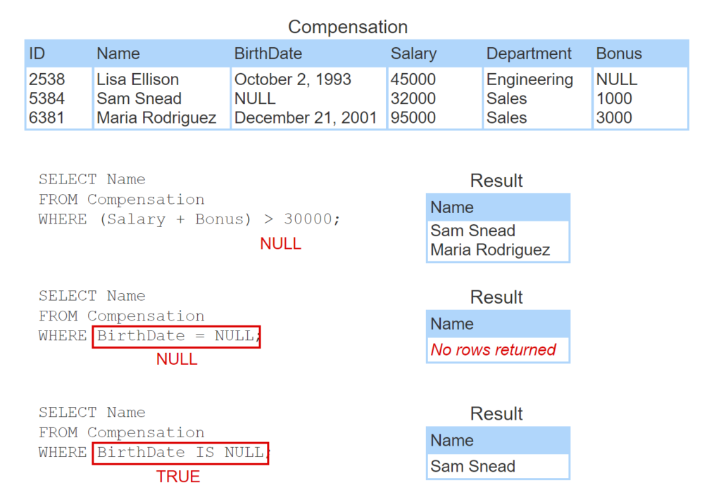
1. Lisa Ellison’s Bonus is NULL. As a result, Salary + Bonus is NULL and (Salary + Bonus) > 30000 is NULL.
2. The SELECT statement does not select a name from a row when the WHERE clause is NULL, so Lisa Ellison is not selected.
3. The = comparison operator returns NULL when either or both operands are NULL, so the WHERE clause evaluates to NULL for Sam Snead.
4. BirthDate IS NULL returns TRUE for Sam Snead, so Sam Snead is selected.

NULL and aggregate functions

SQL statements also contain aggregate functions. An aggregate function operates on numeric values from multiple rows, including only rows selected by the WHERE clause. Aggregate functions include:

• SUM, which returns the total of selected values.
• AVG, which returns the average of selected values.
• MAX, which returns the largest selected value.
• MIN, which returns the smallest selected value.

SUM, AVG, MIN, and MAX ignore NULL values.

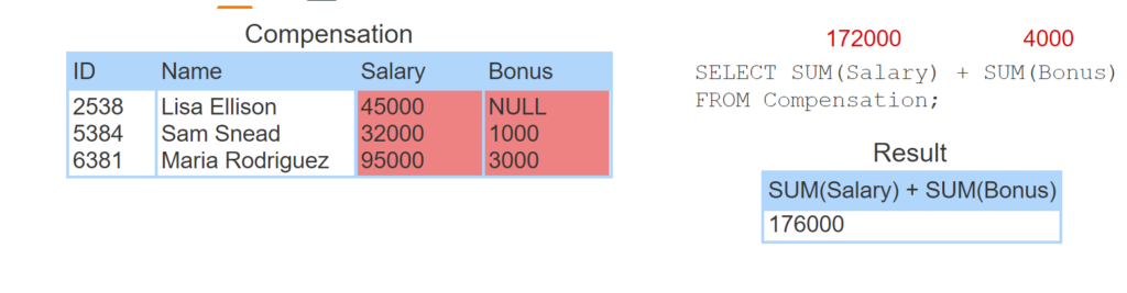
1. The SELECT statement has no WHERE clause, so all rows are selected.
2. SUM(Salary) returns 172000.
3. SUM(Bonus) ignores NULL and returns 4000.
4. The SELECT statement returns 172000 + 4000.

Ignoring NULL can generate surprising results. At first glance, SUM(Salary) + SUM(Bonus) seems equivalent to SUM(Salary + Bonus). However, the results may differ when NULL is present.

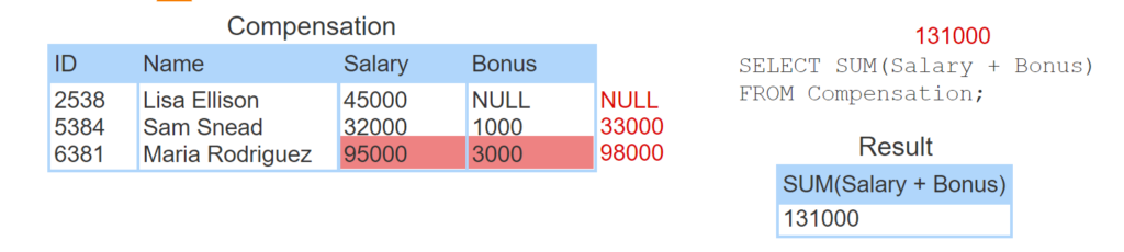
1. 45000 + NULL is NULL.
2. Salary + Bonus is computed for the remaining rows.
3. SUM ignores NULL and returns 33000 + 98000.

NULL logic

In traditional mathematical logic, expressions are always TRUE or FALSE. When NULL is present, however, a logical expression may be either TRUE, FALSE, or NULL. NULL indicates the value of a logical expression is uncertain. Ex:

• TRUE AND TRUE is TRUE.
• TRUE AND FALSE is FALSE.
• TRUE AND NULL is NULL.

The value of logical expressions containing NULL operands is defined in truth tables.

Figure 2.3.1: MySQL truth tables.

x	y	x AND y	x OR y
TRUE	NULL	NULL	TRUE
NULL	TRUE
FALSE	NULL	FALSE	NULL
NULL	FALSE
NULL	NULL	NULL	NULL

x	NOT x
NULL	NULL

MySQL does not have a special data type for logical values. Internally, MySQL represents FALSE as 0 and TRUE as 1. In query results, FALSE and TRUE are also displayed as 0 and 1.

Since null logic is not standardized in mathematics, implementation details vary. Ex: Oracle Database displays a NULL logical expression as UNKNOWN.

2.4 Primary and foreign keys

Primary keys

A primary key is a column, or group of columns, used to identify a row. In the Employee table below, the primary key is ID because each employee has a unique employee ID. The primary key usually appears on the table’s left side, but the primary key’s position is not significant to the database. In this material, a solid circle (●) precedes the primary key in table examples.

Table 2.4.1: Employee table with primary key ID.

ID	Name	Salary
2538	Lisa Ellison	45000
5384	Sam Snead	30500
6381	Maria Rodriguez	92300

Often, primary key values are used in the WHERE clause to select a specific row.

Figure 2.4.1: Primary key used to select a specific employee.

SELECT Name
FROM Employee
WHERE ID = 5384;

Sam Snead

The primary key is specified in SQL when the table is created. If a table contains several unique columns, any unique column may be specified.

Primary keys obey two rules:

• Values must be unique within the column. This rule ensures that each value identifies at most one row.
• Values may not be NULL. This rule ensures that each value identifies at least one row.

Together, the two rules ensure that each primary key value identifies exactly one row.

Composite primary keys

Sometimes multiple columns are necessary to identify a row. A simple primary key consists of a single column. A composite primary key consists of multiple columns. Composite primary keys are denoted with parentheses. Ex: (ColumnA, ColumnB).

In the Family table below, an employee may have several family members, so employee ID is not unique. The composite primary key consists of the ID and Number columns, denoted (ID, Number).

In a minimal primary key, all columns are necessary for uniqueness. When any column is removed from a minimal composite primary key, the resulting simple or composite column is no longer unique.

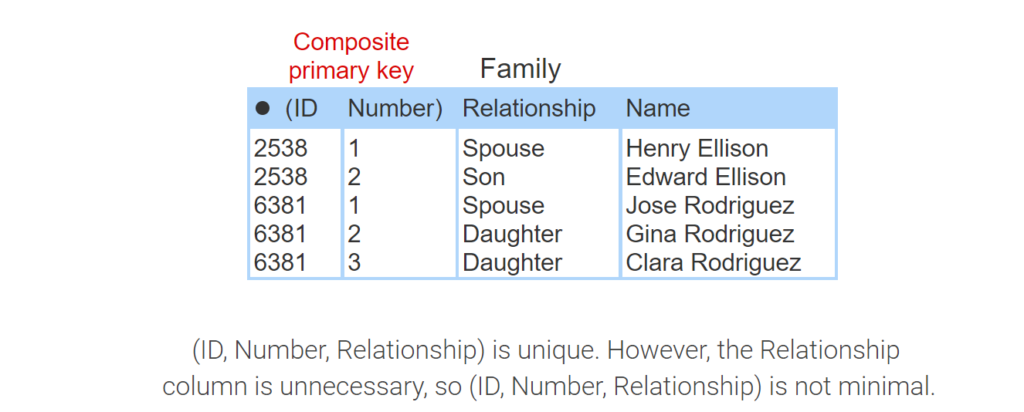
1. ID is not unique in the Family table.
2. ID and Number together is unique, so (ID, Number) is a composite primary key.
3. (ID, Number, Relationship) is unique. However, the Relationship column is unnecessary, so (ID, Number, Relationship) is not minimal.

Composite primary keys obey three rules:

1. Column values, when grouped together, must be unique. Ex: The combination (2538, 1) is unique within (ID, Number).
2. Columns may not contain NULL.
3. Composite primary keys must be minimal.

The first two rules are similar to simple primary keys. Simple primary keys are necessarily minimal, since no column can be removed from a simple key.

Foreign keys

A foreign key is a column, or group of columns, that refer to a primary key. Non-NULL foreign key values must match some value of the primary key. The data types of the foreign and primary keys must be the same, but the names may be different. In this material, an empty circle (○) precedes foreign keys in table examples.

The Manager column of the Department table below refers to the ID column of Employee, so Manager is a foreign key. Both columns have an integer data type, but ID and Manager are different names.

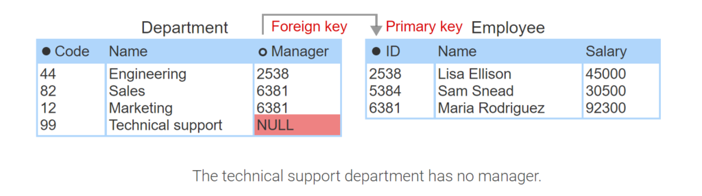
1. The Department table’s Manager column is a foreign key that refers to the primary key ID in the Employee table.
2. Lisa Ellison manages the engineering department.
3. Maria Rodriguez manages the sales and marketing departments.
4. The technical support department has no manager.

Foreign keys do not obey the same rules as primary keys:

• Foreign key values may be repeated. Ex: Sales and Marketing have the same manager.
• Foreign key values may be NULL. Ex: Technical support currently has no manager.
• Non-NULL foreign key values must match some primary key value.

Special cases

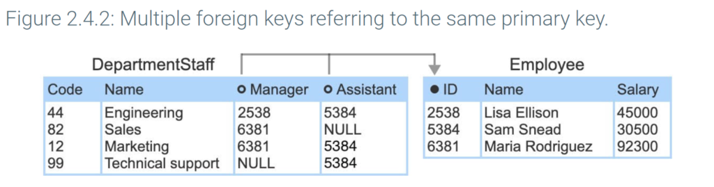
Several foreign keys may refer to the same primary key. In the DepartmentStaff table, the Manager and Assistant foreign keys both refer to ID, the primary key of Employee.

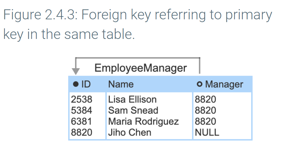
A foreign key may refer to a primary key in the same table. In the EmployeeManager table, the Manager foreign key refers to the ID primary key.

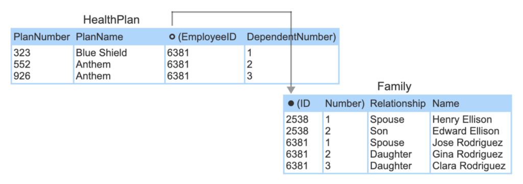
A foreign key that refers to a composite primary key must also be composite. In the HealthPlan table, (EmployeeID, DependentNumber) is a composite foreign key that refers to the Family table’s primary key.

2.5 Referential integrity

Referential integrity rules

A fully NULL foreign key is a simple or composite foreign key in which all columns are NULL. Referential integrity requires that all foreign key values must either be fully NULL or match some primary key value.

In a relational database, foreign keys must obey referential integrity at all times. Occasionally, data entry errors or incomplete data result in referential integrity violations. Violations must be corrected before data is stored in the database.

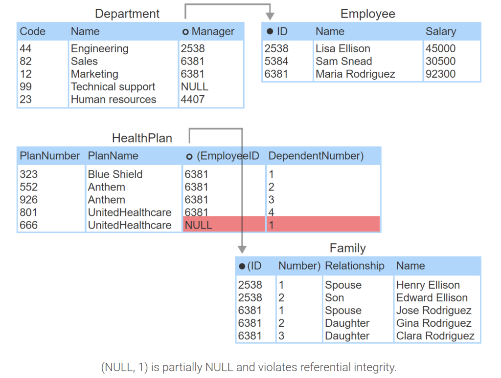
1. 4407 does not match any value in ID and violates referential integrity.
2. (6381, 4) does not match any value in (ID, Number) and violates referential integrity.
3. (NULL, 1) is partially NULL and violates referential integrity.

Referential integrity violations

Referential integrity can be violated in four ways:

1. A primary key is updated.
2. A foreign key is updated.
3. A row containing a primary key is deleted.
4. A row containing a foreign key is inserted.

Only these four operations can violate referential integrity. Primary key inserts and foreign key deletes cannot violate referential integrity.

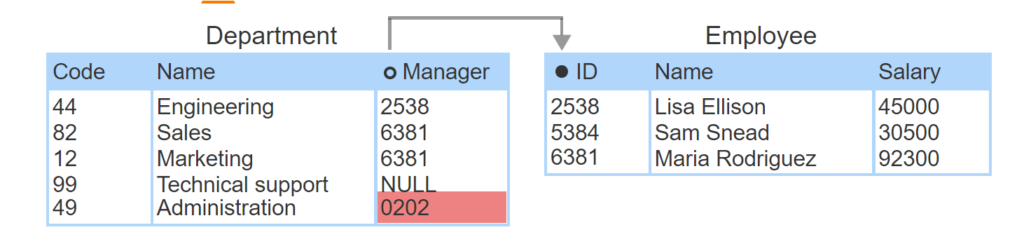
1. Primary key update violates referential integrity.
2. Foreign key update violates referential integrity.
3. Primary key delete violates referential integrity.
4. Foreign key insert violates referential integrity.

Referential integrity actions

An insert, update, or delete that violates referential integrity can be corrected manually. A database user can correct an invalid foreign key with an update, or create a matching primary key with an insert. However, manual corrections are time-consuming and error-prone.

Databases can automatically correct referential integrity violations with any of four actions, which are specified in SQL when creating a table with a foreign key:

• RESTRICT rejects an insert, update, or delete that violates referential integrity.
• SET NULL sets invalid foreign keys to NULL.
• SET DEFAULT sets invalid foreign keys to a default primary key value, specified in SQL.
• CASCADE propagates primary key changes to foreign keys.

CASCADE behaves differently for primary key updates and deletes. If a primary key is deleted, rows containing matching foreign keys are deleted. If a primary key is updated, matching foreign keys are updated to the same value.

Most databases support all four actions for primary key updates and deletes. For foreign key inserts and updates, most databases support only RESTRICT. Databases have the following additional limitations:

• RESTRICT is applied when no action is specified.
• SET NULL cannot be used when a foreign key is not allowed NULL values.
• The value specified for SET DEFAULT must be a valid primary key

.

2.6 Inner and outer joins

Joins

In relational databases, reports are commonly generated from data in multiple tables. Multi-table reports are written with join statements.

A join is a SELECT statement that combines data from two tables, known as the left table and right table, into a single result. The tables are combined by comparing columns from the left and right tables, usually with the = operator. The columns must have comparable data types.

Usually, a join compares a foreign key of one table to the primary key of another. However, a join can compare any columns with comparable data types.

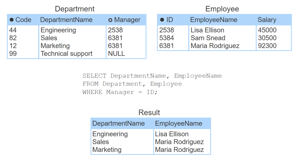
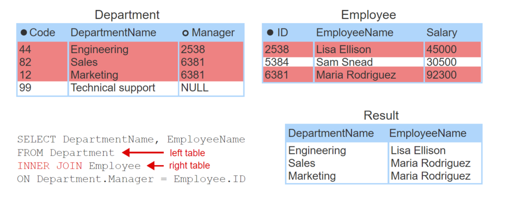
1. The join query displays department names and managers.
2. Department is the left table. Employee is the right table.
3. The query selects rows for which the foreign key Manager equals the primary key ID.
4. Lisa Ellison manages the Engineering department. Maria Rodriguez manages the Sales and Marketing departments.
5. Sam Snead’s ID does not appear in the Manager column, so Sam Snead does not appear in the result.
6. Technical support has a NULL manager, so Technical support does not appear in the result.

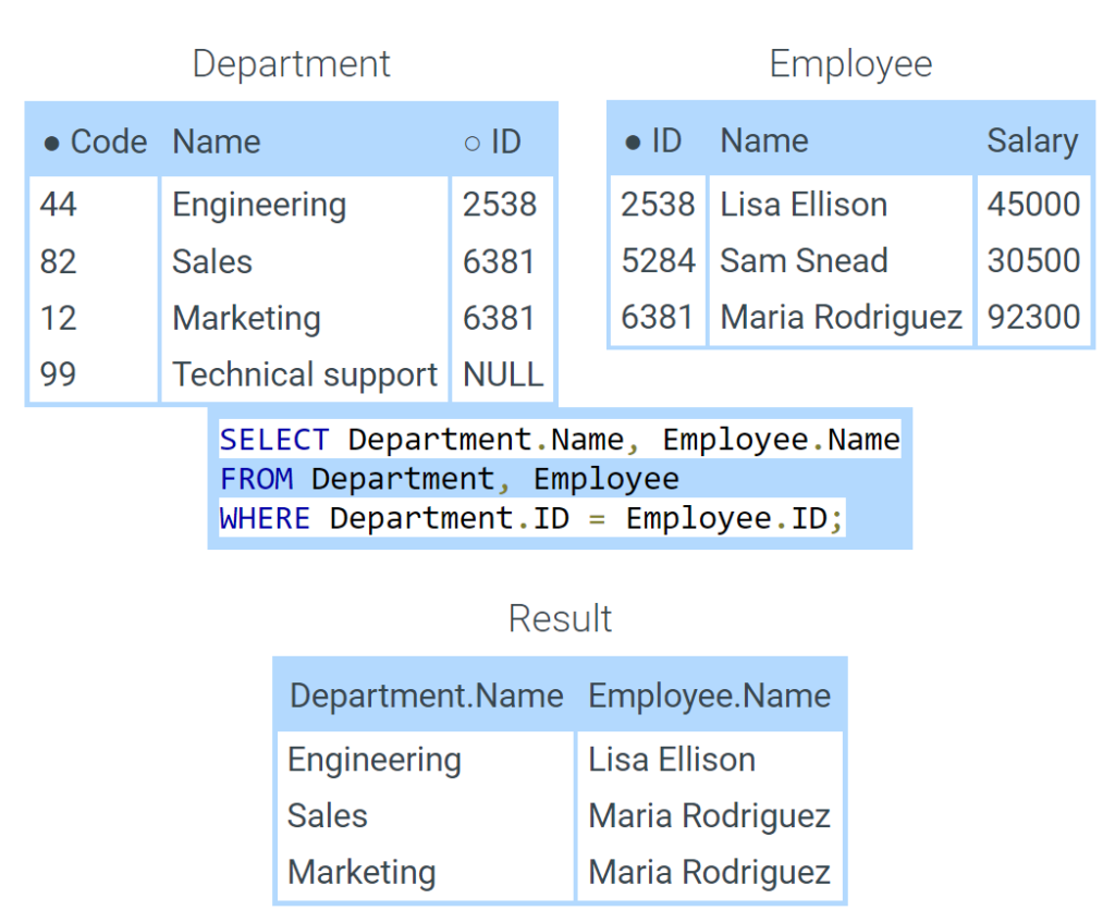
Occasionally, the join tables contain columns with the same name. When columns with the same name appear in a query, the names must be distinguished with a prefix. The prefix is the table name followed by a period. Ex: in the figure below, Department and Employee both have columns Name and ID, which appear with prefixes in the join query.

Inner and outer joins

Matching left and right table rows always appear in a join. In some cases, the database user may also want to see unmatched rows from left, right, or both tables. To enable all cases, relational databases have four types of joins:

• An inner join selects only matching left and right table rows.
• A left join selects all left table rows, but only matching right table rows.
• A right join selects all right table rows, but only matching left table rows.
• A full join selects all left and right table rows, regardless of match.

An outer join is any join that selects unmatched rows, including left, right, and full joins. The result table of an outer join may contain unknown values. In the result table of a left join, for example, unmatched left table values are paired with unknown right table values. These unknown values appear as NULL in the result table.

Inner, left, right, and full joins are written with keywords INNER JOIN, LEFT JOIN, RIGHT JOIN, and FULL JOIN, as in the animations below. The ON clause specifies the join columns. The left table appears in the FROM clause, and the right table appears in the JOIN clause.

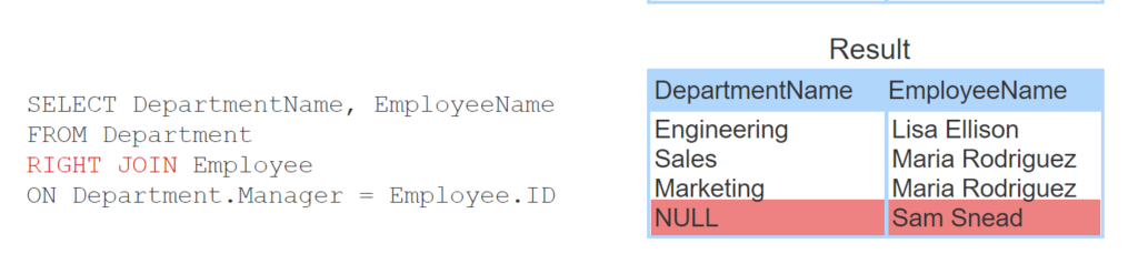
1. Left joins are written with the LEFT JOIN keywords. Unmatched rows from Department, the left table, appear in the result.
2. Right joins are written with the RIGHT JOIN keywords. Unmatched rows from Employee, the right table, appear in the result.

MySQL join syntax differs somewhat from the SQL standard described above. Ex: MySQL does not support the FULL JOIN keyword. For details, see the link in ‘Exploring Further’, below.

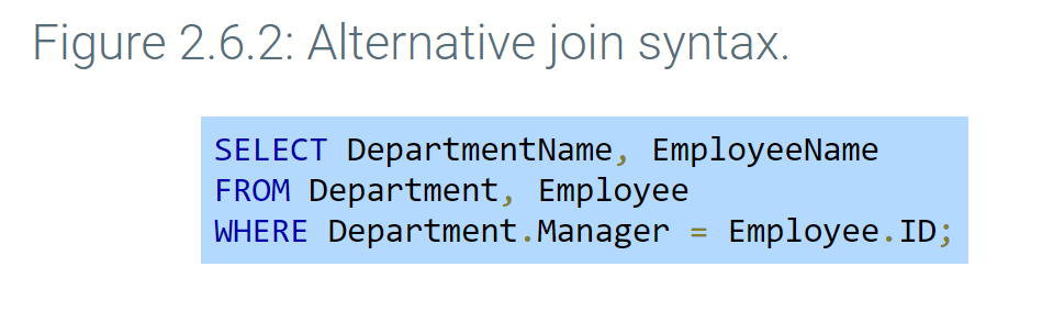
Joins can be written without the JOIN and ON keywords. Ex: The query below executes an inner join. However, using JOIN and ON makes the join explicit and is good practice.

Special cases

Relational databases have several special joins. Most special joins are used infrequently for unusual reporting needs. All of the following special joins can be implemented as an inner, left, right, or full join:

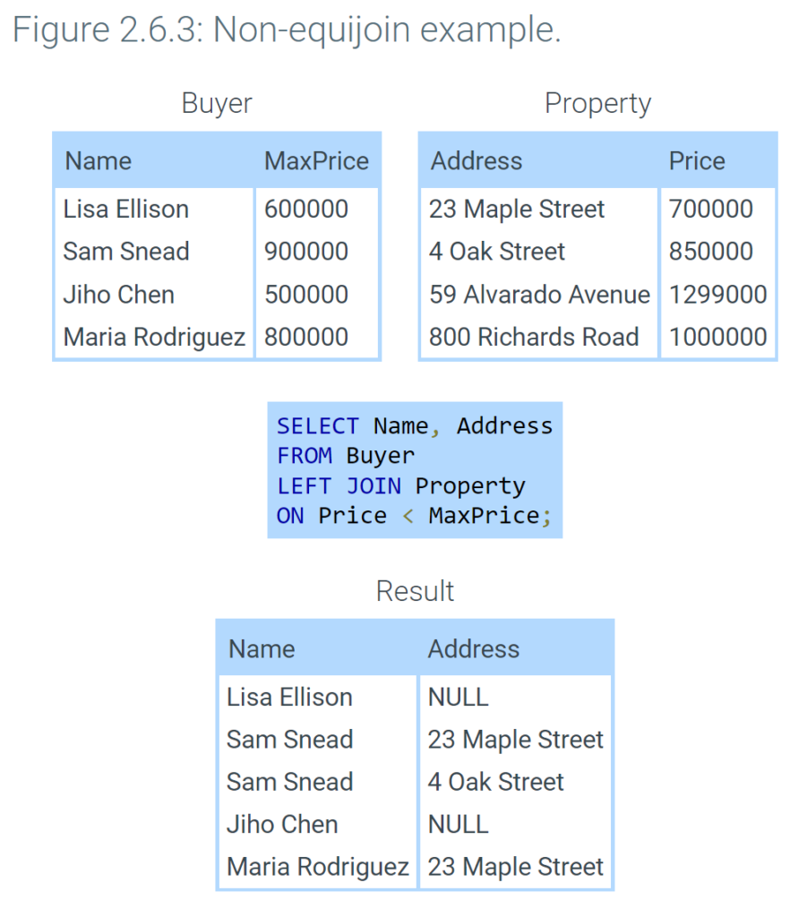
An equijoin compares columns of two tables with the = operator. Most joins are equijoins, including the examples above.

A non-equijoin compares columns with an operator other than =, such as <, >. In the example below, a non-equijoin selects all buyers along with properties priced below the buyer’s maximum price.

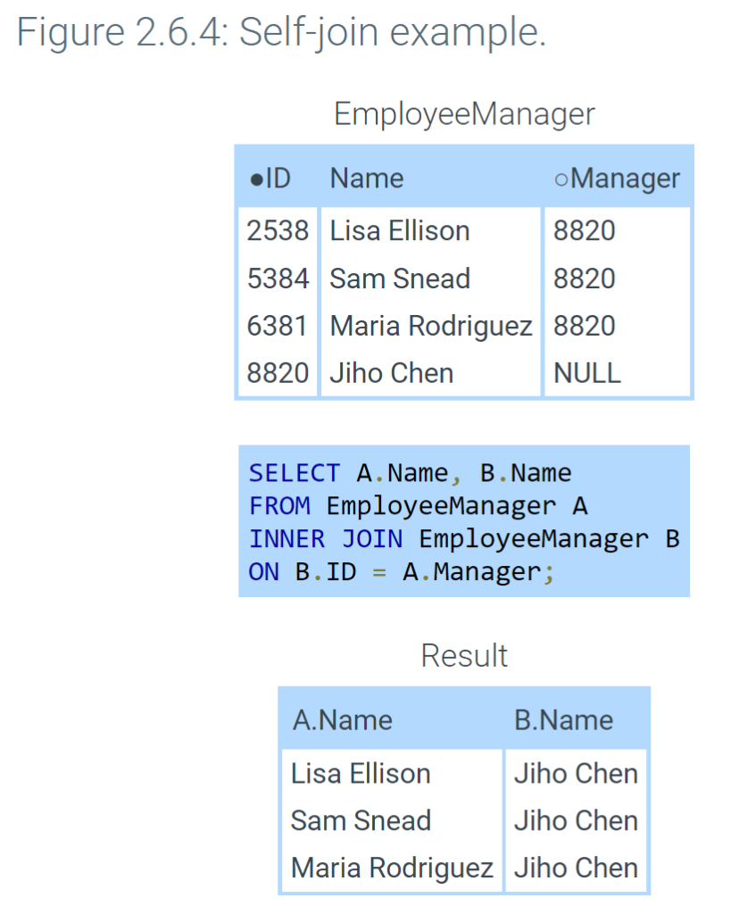
In a self-join, a table is joined to itself. A self-join can compare any columns of a table, as long as the columns have comparable data types. If a foreign key and the referenced primary key are in the same table, a self-join might compare key columns.

In a self-join, aliases are necessary to distinguish left and right tables. An alias is a temporary name assigned to a column or table. In the example below, A is the left table’s alias, and B is the right table’s alias. A.Name is the Name column of the left table, representing the employee. B.Name is the Name column of the right table, representing the employee’s manager. The result shows employees along with each employee’s manager.

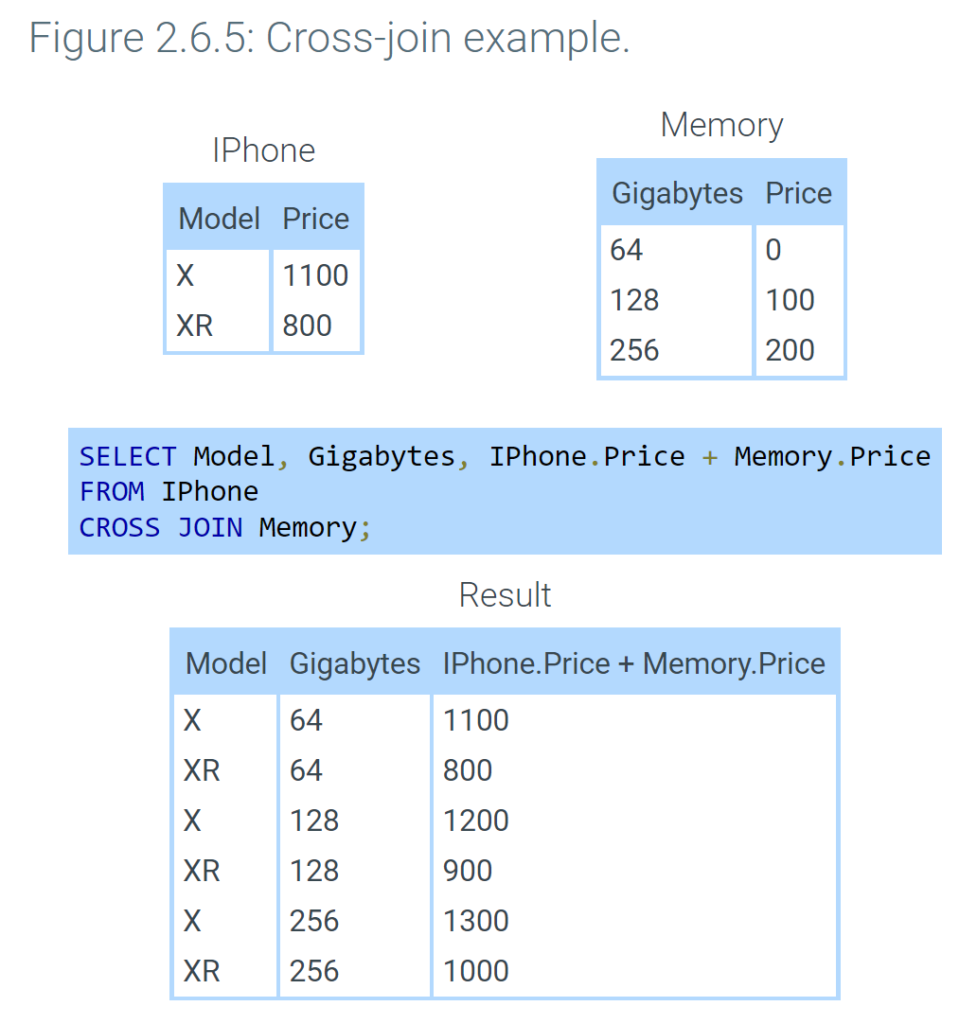
A cross-join combines two tables without comparing columns. A cross-join uses the CROSS JOIN keywords without a WHERE or ON clause. As a result, all possible combinations of rows from both tables appear in the result.

In the example below, all configurations of iPhone models and memory appear, along with total price.

2.7 View tables

Creating views

Table design is optimized for a variety of reasons, such as minimal storage, fast query execution, and support for structural and business rules. Occasionally, the design is not ideal for database users and programmers. Ex: The Employee table may contain personal information, such as name, marital status, and birth date. A separate Address table may contain employee addresses. This design allows several employees to share the same address. Human resources staff, however, may prefer to see personal and address information in one table rather than two.

View tables solve this problem. Views restructure table columns and data types without changes to the underlying database design.

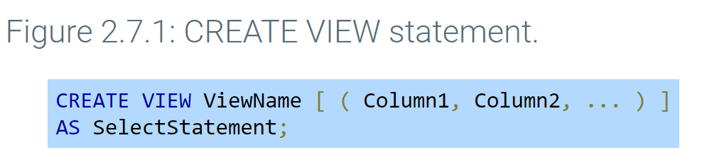
A view table is a table name associated with a SELECT statement, called the view query. The CREATE VIEW statement creates a view table and specifies the view name, query, and, optionally, column names. If column names are not specified, column names are the same as in the view query result table.

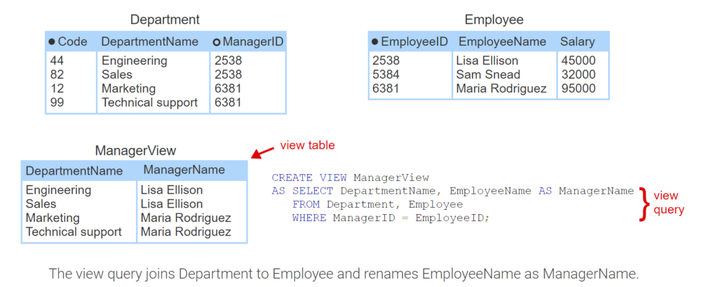
1. Department contains a foreign key that identifies the manager in Employee.
2. CREATE VIEW creates a view table called ManagerView. The view query is a SELECT statement.
3. The view query joins Department to Employee and renames EmployeeName as ManagerName.

Querying views

A table specified in the view query’s FROM clause is called a base table. Unlike base table data, view table data is not normally stored. Instead, when a view table appears in an SQL statement, the view query is merged with the SQL query. The database executes the merged query against base tables.

In some databases, view data can be stored. A materialized view is a view for which data is stored at all times. Whenever a base table changes, the corresponding view tables can also change, so materialized views must be refreshed. To avoid the overhead of refreshing views, MySQL and many other databases do not support materialized views.

TerminologyA view can be defined on other view tables when the view query FROM clause includes additional view tables. In this case, the additional view tables are not base tables. Base tables are always source tables, created as tables rather than as views.

TerminologyA view can be defined on other view tables when the view query FROM clause includes additional view tables. In this case, the additional view tables are not base tables. Base tables are always source tables, created as tables rather than as views.

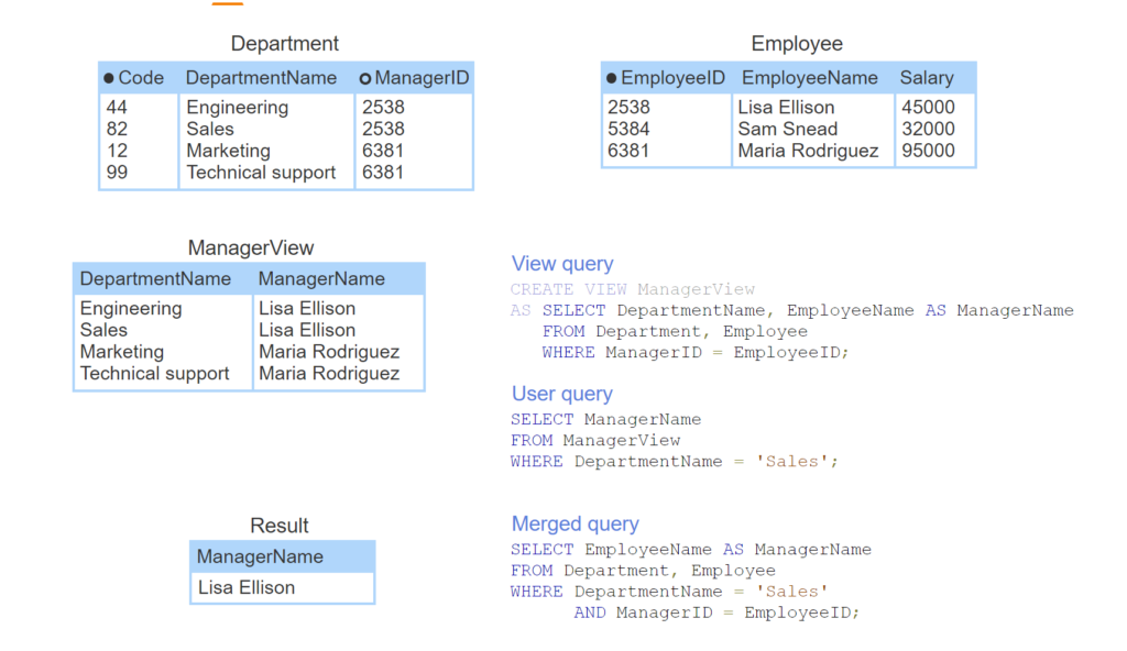
1. A view query joins the base tables Department to Employee to create the ManagerView view table.
2. The user submits a query against the ManagerView table.
3. The database merges the user query with the view query.
4. The merged query is executed against base tables. The result shows the manager of Sales.

Advantages of views

View tables have several advantages:

• Protect sensitive data. A table may contain sensitive data. Ex: The Employee table contains compensation columns such as Salary and Bonus. A view can exclude sensitive columns but include all other columns. Authorizing users and programmers access to the view but not the underlying table protects the sensitive data.
• Save complex queries. Complex or difficult SELECT statements can be saved as a view. Database users can reference the view without writing the SELECT statement.
• Save optimized queries. Often, the same result table can be generated with equivalent SELECT statements. Although the results of equivalent statements are the same, performance may vary. To ensure fast execution, the optimal statement can be saved as a view and distributed to database users.

For the above reasons, views are supported in all relational databases and are frequently created by database administrators. Database users need not be aware of the difference between view and base tables.

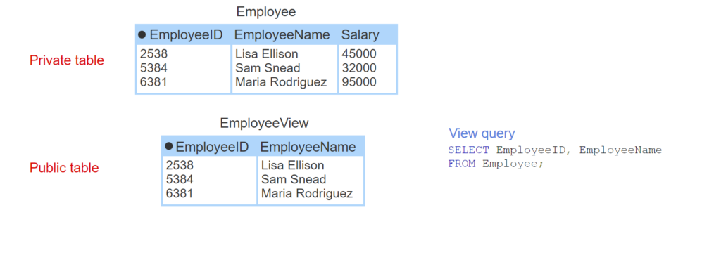
1. The Employee table contains sensitive salary data.
2. The EmployeeView query hides salary data.
3. Only Human Resources staff can access Employee. Anyone can access EmployeeView.

Updating views

View tables are commonly used in SELECT statements. Using views in INSERT, UPDATE, and DELETE statements is problematic:

• Primary keys. If a base table primary key does not appear in a view, an insert to the view generates a NULL primary key value. Since primary keys may not be NULL, the insert is not allowed.
• Aggregate values. A view query may contain aggregate functions such as AVG() or SUM(). One aggregate value corresponds to many base table values. An update or insert to the view may create a new aggregate value, which must be converted to many base table values. The conversion is undefined, so the insert or update is not allowed.
• Join views. In a join view, foreign keys of one base table may match primary keys of another. A delete from a view might delete foreign key rows only, or primary key rows only, or both the primary and foreign key rows. The effect of the join view delete is undefined and therefore not allowed.

The above examples illustrate just a few of many potential problems of view updates. As a result, relational databases either disallow or severely limit view table inserts, updates, and deletes. Regardless of specific database limitations, view updates may have surprising results and should be avoided. Views are best for SELECT statements.

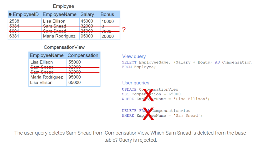
1. The Employee table contains salary and bonus information.
2. Two different employees have the same name but different EmployeeIDs.
3. The CompensationView table contains total compensation.
4. The user query updates Lisa Ellison’s compensation. Lisa Ellison’s new salary and bonus are undefined, so the query is rejected.
5. The user query deletes Sam Snead from CompensationView. Which Sam Snead is deleted from the base table? Query is rejected.
   

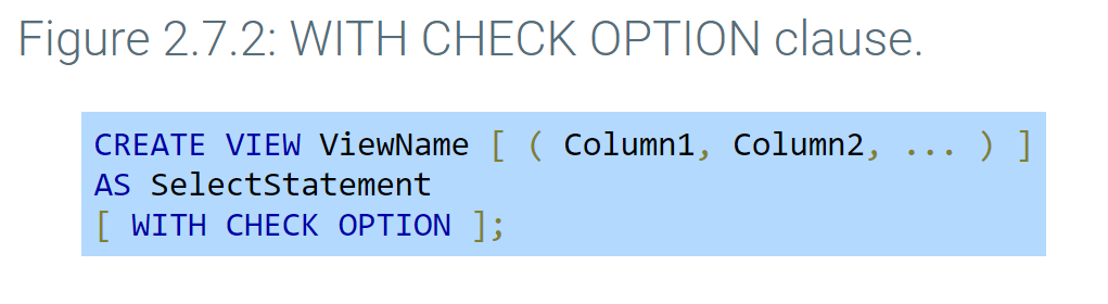
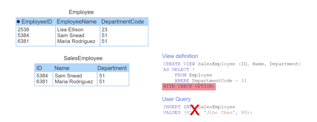
1. Two employees are in department 51, Sales.
2. CREATE VIEW specifies new names for SalesEmployee columns.
3. SalesEmployee view only includes employees in department 51.
4. The user query inserts a new employee in department 80 into the view table.
5. The new employee is inserted into Employee but is not in department 51 and does not appear in the view table.
6. WITH CHECK OPTION prevents inserts and updates that do not satisfy the view query WHERE clause.

2.8 Relational algebra

Operations and expressions

In his original paper on the relational model, E. F. Codd introduced formal operations for manipulating tables. Codd’s operations, called relational algebra, have since been refined and are the theoretical foundation of SQL. Relational algebra is primarily of theoretical interest but does have practical application in compiling SQL queries.

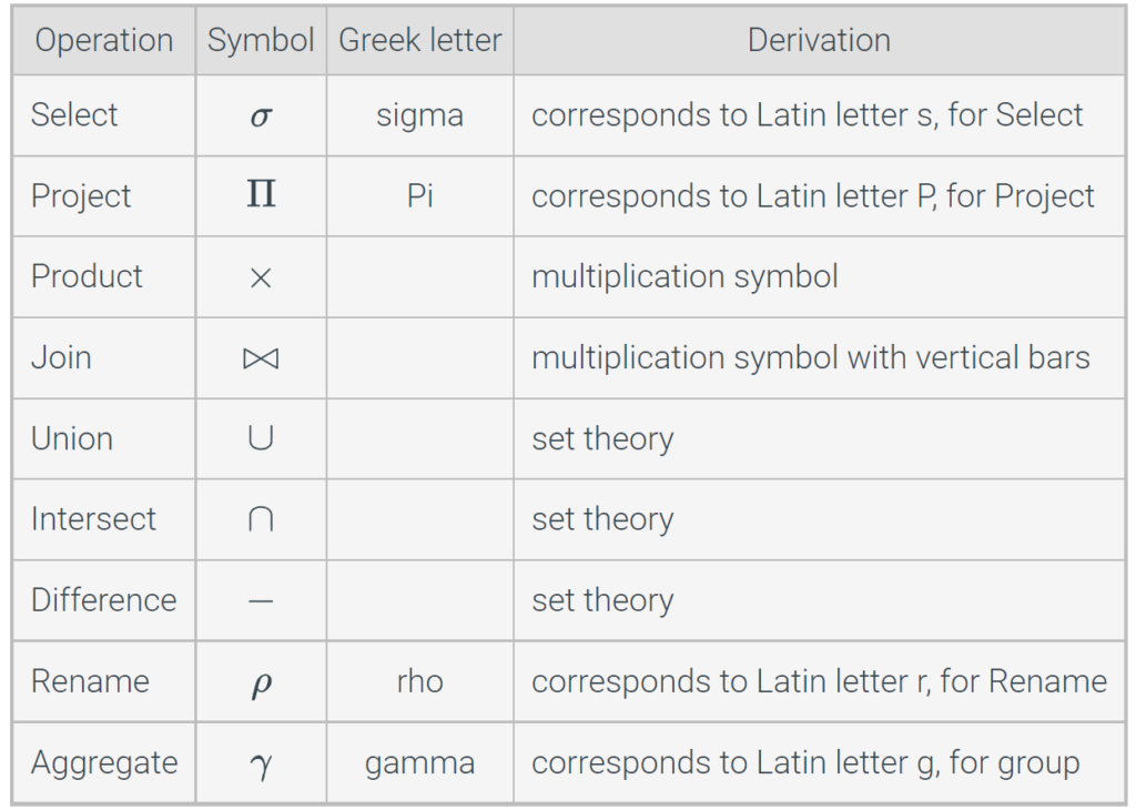
Relational algebra has nine operations. Each operation is denoted with a special symbol, often a letter of the Greek alphabet. Operation symbols can be combined with tables in expressions, just as + – × / can be combined with numbers in arithmetic expressions. Each relational algebra expression is equivalent to an SQL query and defines a single result table.

Table 2.8.1: Relational algebra operations.

Additional operations – Relational algebra is not standardized. Some authors include additional operations, such as assign and divide. Variations of the join operation, such as inner join, full join, and equijoin, are sometimes considered distinct operations.

Select and project

The select operation selects table rows based on a logical expression. The select operation is written asσexpression(Table)and is equivalent to SELECT * FROM Table WHERE expression.

The project operation selects table columns. The project operation is written asΠ(Column1,Column2,…)(Table)and is equivalent to SELECT Column1, Column2, ... FROM Table.

Product and join

The product operation combines two tables into one result. The result includes all columns and all combinations of rows from both tables. The product operation is written asTable1×Table2and is equivalent to SELECT * FROM Table1 CROSS JOIN Table2. If Table1 has n₁ rows and Table2 has n₂ rows, then the product has n₁ × n₂ rows.

The join operation, denoted with a “bowtie” symbol, is written asTable1⋈expressionTable2and is identical to a product followed by a select:σexpression(Table1×Table2)The join operation is equivalent to SELECT * FROM Table1 INNER JOIN Table2 ON expression. The join expression is any expression on columns of Table1 and Table2, and is often denoted with the Greek letter theta:Table1⋈θTable2Because of theta notation, the join operation is sometimes called a theta join.

The bowtie symbol ⋈ represents an inner join operation. Left, right, and full joins are represented by symbols ⟕ , ⟖ , and ⟗ , respectively.

Union, intersect, and difference

Compatible tables have the same number of columns with the same data types. Column names may be different. Union, intersect, and difference operate on compatible tables and, collectively, are called set operations.

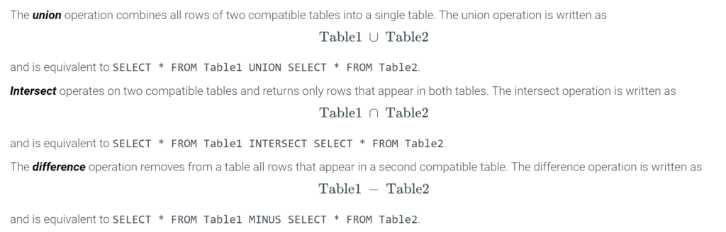
For all three set operations, the result column names are the Table1 column names.

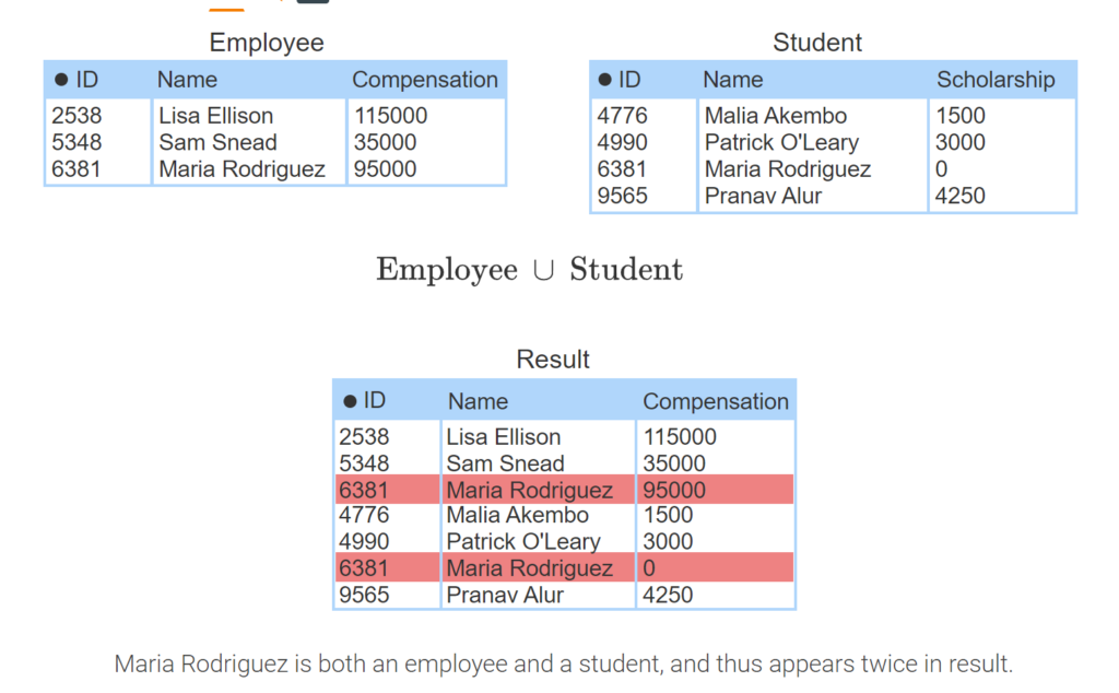
1. A university has separate employee and student tables. The tables are compatible even though the third column names are different.
2. The compatible tables can be combined in a union operation.
3. The result column names are taken from the first table in the union, Employee.
4. Maria Rodriguez is both an employee and a student, and thus appears twice in result.

Set operations in MySQL

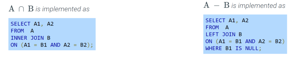
The UNION, INTERSECT, and MINUS keywords are part of the SQL standard. MySQL supports UNION but not INTERSECT and MINUS. In MySQL, the intersect and difference operations can be implemented as joins. Ex: Table A has columns A1 and A2. Table B has columns B1 and B2.

Rename and aggregate

The rename operation specifies new table and column names. The rename operation is written as

If TableName is omitted, only the column names are changed. If (ColumnName1, ColumnName2, … ) is omitted, only the table name is changed.

The aggregate operation applies aggregate functions like SUM(), AVG(), MIN(), and MAX(). The aggregate operation is written asGroupColumnγFunction(Column)(Table)

and is equivalent to SELECT GroupColumn, Function(Column) FROM Table GROUP BY GroupColumn.

If GroupColumn is omitted, the operation is equivalent to SELECT Function(Column) FROM Table and computes a single aggregate value for all rows.

Notation for the aggregate operation varies. In this material, the aggregate operation is denoted with the Greek letter gamma (γ). Some publications use the Latin letter G, the script F (ℱ), or the script A (𝒜).

Query optimization

Relational algebra expressions are equivalent if the expressions operate on the same tables and generate the same result. Ex:

Although the operation order is different, both expressions operate on Employee and define the same result table.

A query optimizer converts an SQL query into a sequence of low-level database actions, called the query execution plan. The query execution plan specifies precisely how to process an SQL statement. A query optimizer is similar to a programming language compiler.

Query optimizers use equivalent expressions to optimize query execution. The query optimizer:

1. Converts a query to a relational algebra expression.
2. Generates equivalent expressions.
3. Estimates the ‘cost’ of each operation of each expression.
4. Determines the optimal expression with the lowest total cost.
5. Converts the optimal expression into a query execution plan.

The cost of an operation is a numeric estimate of processing time. The cost estimate usually combines both storage media access and computation time in a single measure. The animation below illustrates cost as the number of rows read. In practice, query optimizers use more sophisticated cost measures.

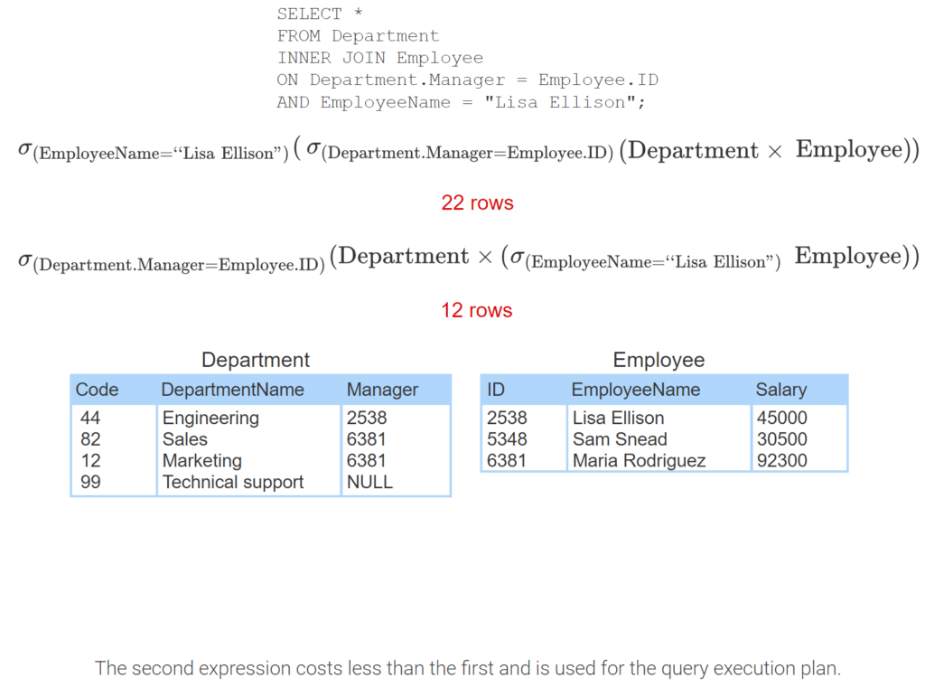
1. The query selects departments managed by Lisa Ellison.
2. In relational algebra, the query is a join followed by a select.
3. The join operation is equivalent to a product followed by a select.
4. The product reads 4 Department rows and 3 Employee rows. The first select reads 12 rows. The second select reads 3 rows.
5. An equivalent expression first selects Lisa Ellison from Employee.
6. The first select reads 3 rows. The product reads 4 Department rows and 1 Employee row. The second select reads 4 rows.
7. The second expression costs less than the first and is used for the query execution plan.