7.1 Algorithms
Problem solving and algorithms
Programs solve problems. Before writing a program, a programmer must first create an algorithm to correctly solve the given problem. An algorithm is a sequence of steps that solves a problem, generating correct output for any valid input values. Ensuring an algorithm’s correctness is a key job for a programmer.
Introduction to algorithm efficiency
Algorithms differ in various features. One feature is algorithm time efficiency: The number of calculations required to solve a problem. For the same problem, some algorithms may be much more time efficient than others.
Simple programs are more likely to be correct, and correctness is always most important. Efficient algorithms tend to be less simple, so programmers should consider efficiency only when needed, like when dealing with very large data sets that result in slow program execution.
7.2 Introduction to algorithms
Algorithms
An algorithm describes a sequence of steps to solve a computational problem or perform a calculation. An algorithm can be described in English, pseudocode, a programming language, hardware, etc. A computational problem specifies an input, a question about the input that can be answered using a computer, and the desired output.
Practical applications of algorithms
Computational problems can be found in numerous domains, including e-commerce, internet technologies, biology, manufacturing, transportation, etc. Algorithms have been developed for numerous computational problems within these domains.
A computational problem can be solved in many ways, but finding the best algorithm to solve a problem can be challenging. However, many computational problems have common subproblems, for which efficient algorithms have been developed. The examples below describe a computational problem within a specific domain and list a common algorithm (each discussed elsewhere) that can be used to solve the problem.Table 7.2.1: Example computational problems and common algorithms.
| Application domain | Computational problem | Common algorithm |
|---|---|---|
| DNA analysis | Given two DNA sequences from different individuals, what is the longest shared sequence of nucleotides? | Longest common substring: The longest common substring algorithm determines the longest common substring that exists in two inputs strings. DNA sequences can be represented using strings consisting of the letters A, C, G, and T to represent the four different nucleotides. |
| Search engines | Given a product ID and a sorted array of all in-stock products, is the product in stock and what is the product’s price? | Binary search: The binary search algorithm is an efficient algorithm for searching a list. The list’s elements must be sorted and directly accessible (such as an array). |
| Navigation | Given a user’s current location and desired location, what is the fastest route to walk to the destination? | Dijkstra’s shortest path: Dijkstra’s shortest path algorithm determines the shortest path from a start vertex to each vertex in a graph. The possible routes between two locations can be represented using a graph, where vertices represent specific locations and connecting edges specify the time required to walk between those two locations. |
Efficient algorithms and hard problems
Computer scientists and programmers typically focus on using and designing efficient algorithms to solve problems. Algorithm efficiency is most commonly measured by the algorithm runtime, and an efficient algorithm is one whose runtime increases no more than polynomially with respect to the input size. However, some problems exist for which an efficient algorithm is unknown.
NP-complete problems are a set of problems for which no known efficient algorithm exists. NP-complete problems have the following characteristics:
- No efficient algorithm has been found to solve an NP-complete problem.
- No one has proven that an efficient algorithm to solve an NP-complete problem is impossible.
- If an efficient algorithm exists for one NP-complete problem, then all NP-complete problems can be solved efficiently.
By knowing a problem is NP-complete, instead of trying to find an efficient algorithm to solve the problem, a programmer can focus on finding an algorithm to efficiently find a good, but non-optimal, solution.
An efficient algorithm is generally one whose runtime increases no more than polynomially with respective to the input size. In contrast, an algorithm with an exponential runtime is not efficient.
7.3 Algorithm efficiency
Algorithm efficiency
An algorithm describes the method to solve a computational problem. Programmers and computer scientists should use or write efficient algorithms. Algorithm efficiency is typically measured by the algorithm’s computational complexity. Computational complexity is the amount of resources used by the algorithm. The most common resources considered are the runtime and memory usage.
- An algorithm’s computational complexity includes runtime and memory usage.
- Measuring runtime and memory usage allows different algorithms to be compared.
- Complexity analysis is used to identify and avoid using algorithms with long runtimes or high memory usage.
Runtime complexity, best case, and worst case
An algorithm’s runtime complexity is a function, T(N), that represents the number of constant time operations performed by the algorithm on an input of size N. Runtime complexity is discussed in more detail elsewhere.
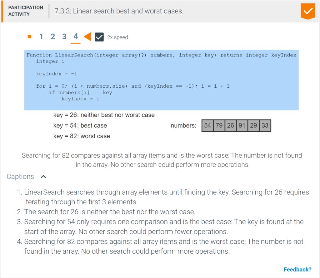
Because an algorithm’s runtime may vary significantly based on the input data, a common approach is to identify best and worst case scenarios. An algorithm’s best case is the scenario where the algorithm does the minimum possible number of operations. An algorithm’s worst case is the scenario where the algorithm does the maximum possible number of operations.
Input data size must remain a variable
A best case or worst case scenario describes contents of the algorithm’s input data only. The input data size must remain a variable, N. Otherwise, the overwhelming majority of algorithms would have a best case of N=0, since no input data would be processed. In both theory and practice, saying “the best case is when the algorithm doesn’t process any data” is not useful. Complexity analysis always treats the input data size as a variable.
Space complexity
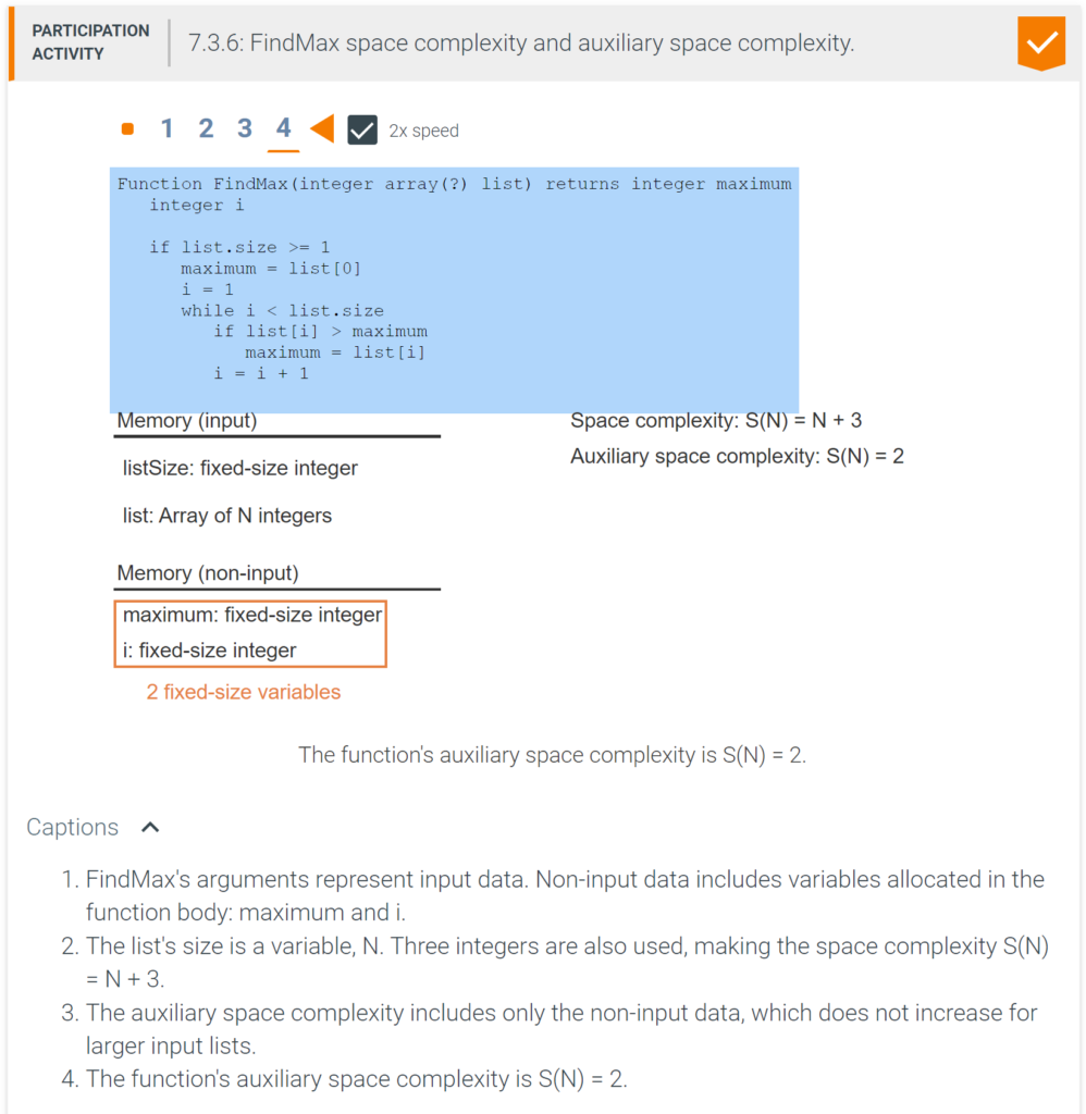
An algorithm’s space complexity is a function, S(N), that represents the number of fixed-size memory units used by the algorithm for an input of size N. Ex: The space complexity of an algorithm that duplicates a list of numbers is S(N) = 2N + k, where k is a constant representing memory used for things like the loop counter and list pointers.
Space complexity includes the input data and additional memory allocated by the algorithm. An algorithm’s auxiliary space complexity is the space complexity not including the input data. Ex: An algorithm to find the maximum number in a list will have a space complexity of S(N) = N + k, but an auxiliary space complexity of S(N) = k, where k is a constant.
7.4 Searching and algorithms
Algorithms
An algorithm is a sequence of steps for accomplishing a task. Linear search is a search algorithm that starts from the beginning of a list, and checks each element until the search key is found or the end of the list is reached.
Algorithm runtime
An algorithm’s runtime is the time the algorithm takes to execute. If each comparison takes 1 µs (1 microsecond), a linear search algorithm’s runtime is up to 1 s to search a list with 1,000,000 elements, 10 s for 10,000,000 elements, and so on. Ex: Searching Amazon’s online store, which has more than 200 million items, could require more than 3 minutes.
An algorithm typically uses a number of steps proportional to the size of the input. For a list with 32 elements, linear search requires at most 32 comparisons: 1 comparison if the search key is found at index 0, 2 if found at index 1, and so on, up to 32 comparisons if the the search key is not found. For a list with N elements, linear search thus requires at most N comparisons. The algorithm is said to require “on the order” of N comparisons.
7.5 Binary search
Linear search vs. binary search
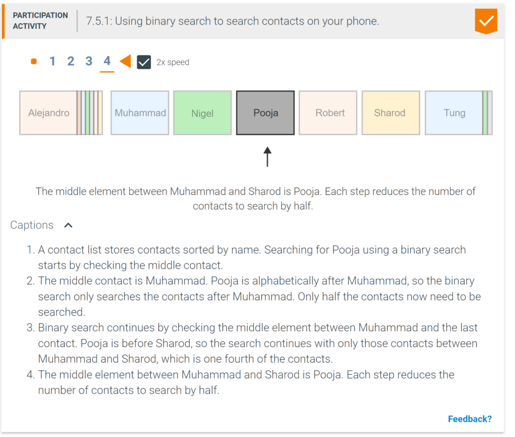
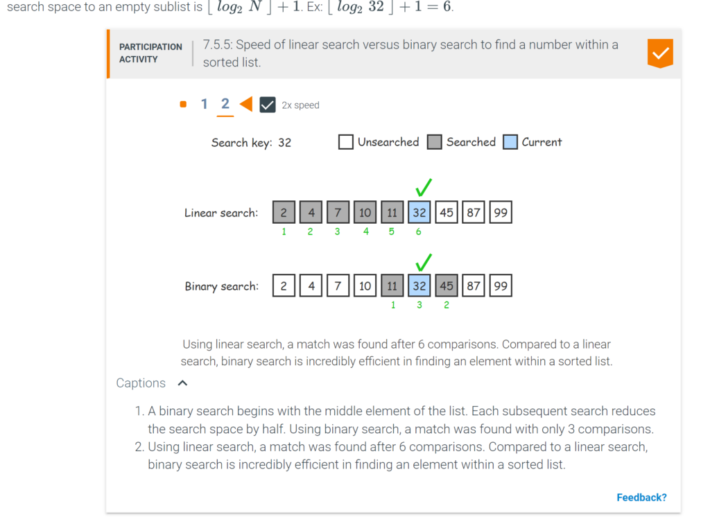
Linear search may require searching all list elements, which can lead to long runtimes. For example, searching for a contact on a smartphone one-by-one from first to last can be time consuming. Because a contact list is sorted, a faster search, known as binary search, checks the middle contact first. If the desired contact comes alphabetically before the middle contact, binary search will then search the first half and otherwise the last half. Each step reduces the contacts that need to be searched by half.
Binary search efficiency
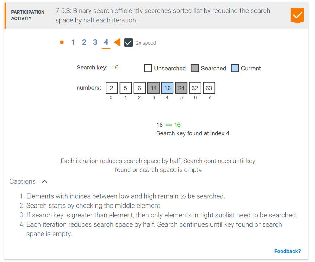
Binary search is incredibly efficient in finding an element within a sorted list. During each iteration or step of the algorithm, binary search reduces the search space (i.e., the remaining elements to search within) by half. The search terminates when the element is found or the search space is empty (element not found). For a 32 element list, if the search key is not found, the search space is halved to have 16 elements, then 8, 4, 2, 1, and finally none, requiring only 6 steps. For an N element list, the maximum number of steps required to reduce the search space to an empty sublist is ⌊log2N⌋+1. Ex: ⌊log232⌋+1=6.
7.6 Sorting: Introduction
Sorting is the process of converting a list of elements into ascending (or descending) order. For example, given a list of numbers (17, 3, 44, 6, 9), the list after sorting is (3, 6, 9, 17, 44). You may have carried out sorting when arranging papers in alphabetical order, or arranging envelopes to have ascending zip codes (as required for bulk mailings).
The challenge of sorting is that a program can’t “see” the entire list to know where to move an element. Instead, a program is limited to simpler steps, typically observing or swapping just two elements at a time. So sorting just by swapping values is an important part of sorting algorithms.
7.7 Heuristics
Heuristics
In practice, solving a problem in the optimal or most accurate way may require more computational resources than are available or feasible. Algorithms implemented for such problems often use a heuristic: A technique that willingly accepts a non-optimal or less accurate solution in order to improve execution speed.
Heuristic optimization
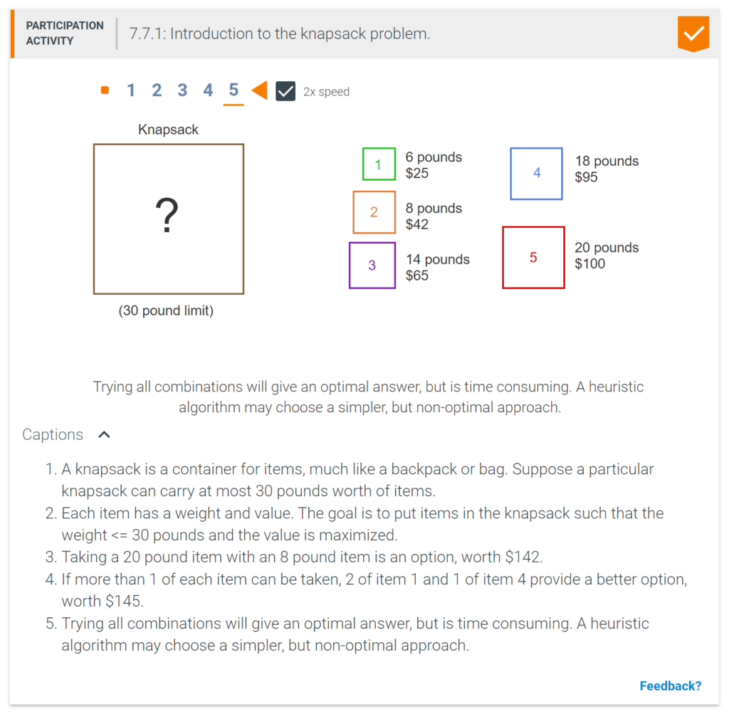
A heuristic algorithm is an algorithm that quickly determines a near optimal or approximate solution. Such an algorithm can be designed to solve the 0-1 knapsack problem: The knapsack problem with the quantity of each item limited to 1.
A heuristic algorithm to solve the 0-1 knapsack problem can choose to always take the most valuable item that fits in the knapsack’s remaining space. Such an algorithm uses the heuristic of choosing the highest value item, without considering the impact on the remaining choices. While the algorithm’s simple choices are aimed at optimizing the total value, the final result may not be optimal.
7.8 Algorithms summary
This chapter’s key points included:
- A programmer must first create a correct algorithm: A sequence of steps to solve a problem.
- For large data, also relevant is an algorithm’s time efficiency: The number of calculations needed to solve a problem.