4.1 Unit 4: Counting and Advanced Counting Techniques

This is the beginning of Unit 4 in this Discrete Mathematics II course.

The material in this unit comprises 19% of the high-stakes assessment and includes such concepts as:

• Bijection, k-to-1, generalize product rules
• Counting permutations and subsets
• Counting multisets
• Generating permutations of a set
• Inclusion-exclusion principle; Binomial Theorem

4.2 Module 13: Counting by Bijections and Products of Sets

This page marks the beginning of Module 13. This module contains three lessons:

• Sum and product rules
• Bijection rule
• Generalized product rule

4.3 Lesson: Sum and product rules

Lesson introduction

A crucial skill in computer science is counting. At first this may seem silly—we all already know how to count, right? 1, 2, 3, 4, etc. However, what if you are trying to count something very large, say the number of possible IDs and passwords, or, if you are feeling hungry, the number of boxes of cookies in a large shipping box? You could count the 72 boxes one by one or you could be more efficient. If you knew how the boxes were stacked—9 boxes in one layer and 8 layers of boxes—you could just multiply the number of boxes in the layers and quickly get the result, 9 x 8 = 72 boxes. The formal name for this method is the “product rule.”

Introduction to counting

Counting, as simple as it may seem initially, is a central topic in discrete mathematics.

The product rule

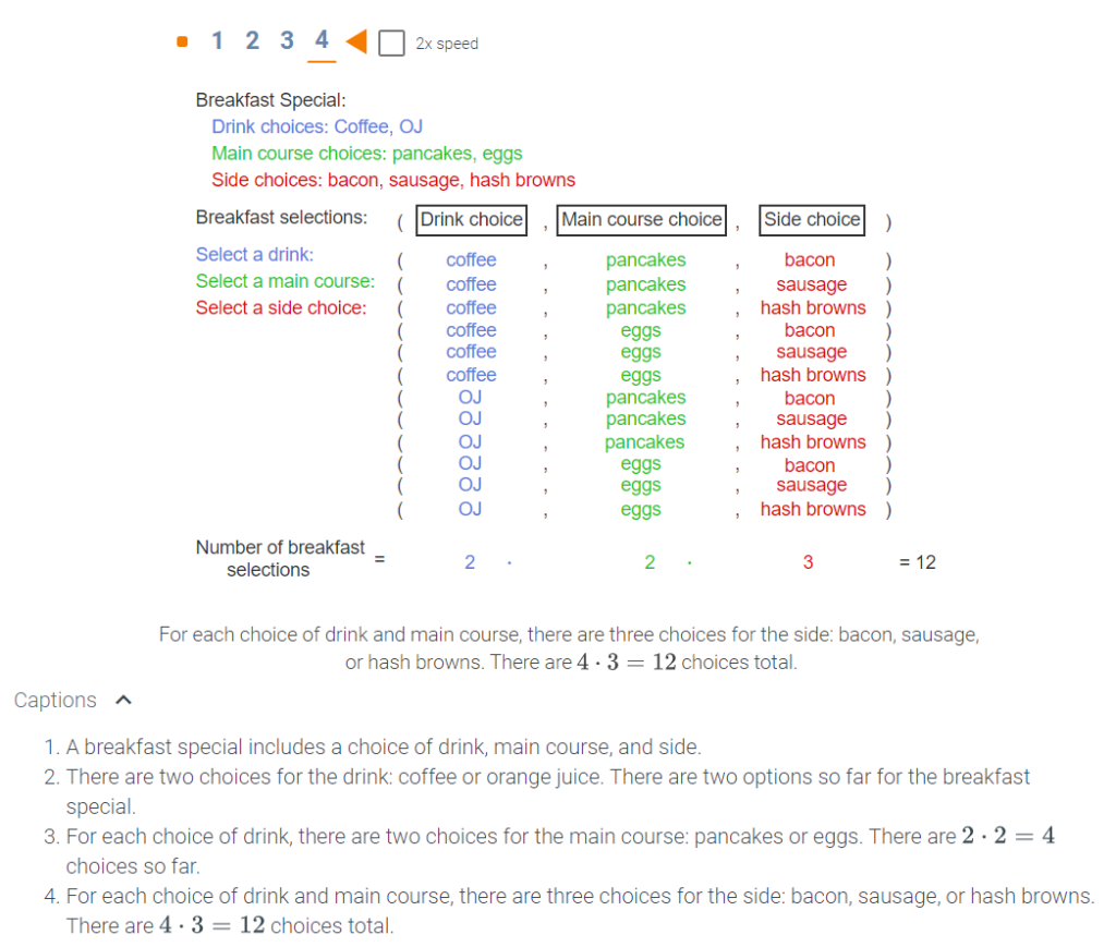
The two most basic rules of counting are the sum rule and the product rule. These two rules applied in different combinations can be used to handle a wide range of counting problems. The product rule provides a way to count sequences. 

Counting strings

If Σ is a set of characters (called an alphabet) then Σⁿ is the set of all strings of length n whose characters come from the set Σ.  For example, if Σ = {0, 1}, then Σ⁶ is the set of all binary strings with 6 bits. The string 011101 is an example of an element in Σ⁶. The strings xxyzx and zyyzy are examples of strings in the set {x, y, z}⁵. The product rule can be applied directly to determine the number of strings of a given length over a finite alphabet:

The sum rule

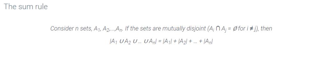
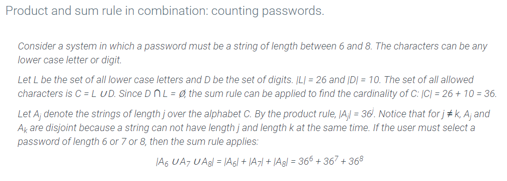
In the breakfast example, the product rule is applied because the customer selects a drink and a main course and a side. In contrast, the sum rule is applied when there are multiple choices but only one selection is made. For example, suppose a customer just orders a drink. The customer selects a hot drink or a cold drink. The hot drink selections are {coffee, hot cocoa, tea}. The cold drink selections are {milk, orange juice}. The total number of choices is 5, namely 3 hot drink choices plus 2 cold drink choices. Here is a formal statement of the sum rule, expressed in terms of sets:

Lesson summary

Now that you have completed this lesson you should be able to solve a counting problem using the sum or product rule. Take a moment to think about what you’ve learned in this lesson:

• The product rule states that the cardinality of individual sequences (number of elements) can be multiplied to determine the total number of possible sequences that could be created from the individual sequences.
  • For example, to determine the number of ways you could choose two cards—a red card and spade—from a standard deck of cards, you would identify the cardinality of each sequence and multiply the numbers. The number of red cards is 26 and the number of spades is 13. In this example there are 338 possible ways to choose two cards. 26 x 13 = 338.
• The sum rule requires a bit more thought than the product rule. When there is an either/or choice to be made, the number of possibilities are calculated by adding the cardinalities. However, if there is any overlap in choices, the number of common choices must be subtracted.
  • For example, to determine the number of ways you could choose either a heart or a face card from a standard deck of cards, you would add the cardinality of the heart cards and the cardinality of face cards. In this example, there are three common choices between these sets. The equation to obtain the result is 13 + 12 – 3 = 22.
• In some cases both the product rule and sum rule are needed to determine the final number of possibilities. For an example, review Participation Activity 4.3.4 .1.4) in this lesson.

4.4 Lesson: Bijection rule

Lesson introduction

In the previous lesson you learned how to use the sum and product rules to count the number of possible sequences that could be determined from individual sequences. But what if you wanted to count one thing by counting another? For example, let’s say you see a pile of shoes from a group of children at the front door. You could determine the number of children (assuming each child had two shoes in the pile) by counting the number of shoes and dividing by two. For this situation you would use a method of counting called “bijection.”

The k-to-1 rule

A group of kids at a slumber party all leave their shoes in a big pile at the door. One way to count the number of kids at the party is to count the number of shoes and divide by 2. Of course, it is important to establish that each kid has exactly one pair of shoes in the pile. Counting kids by counting shoes and dividing by 2 is an example of the k-to-1 rule with k = 2.

k-to-1 correspondence

Let X and Y be finite sets. The function f:X→Y is a k-to-1 correspondence if for every y ∈ Y, there are exactly k different x ∈ X such that f(x) = y.

Lesson summary

Now that you have completed this lesson you should be able to solve a counting problem, including cardinality, using the bijection or k‐to‐1 rule. Take a moment to think about what you’ve learned in this lesson:

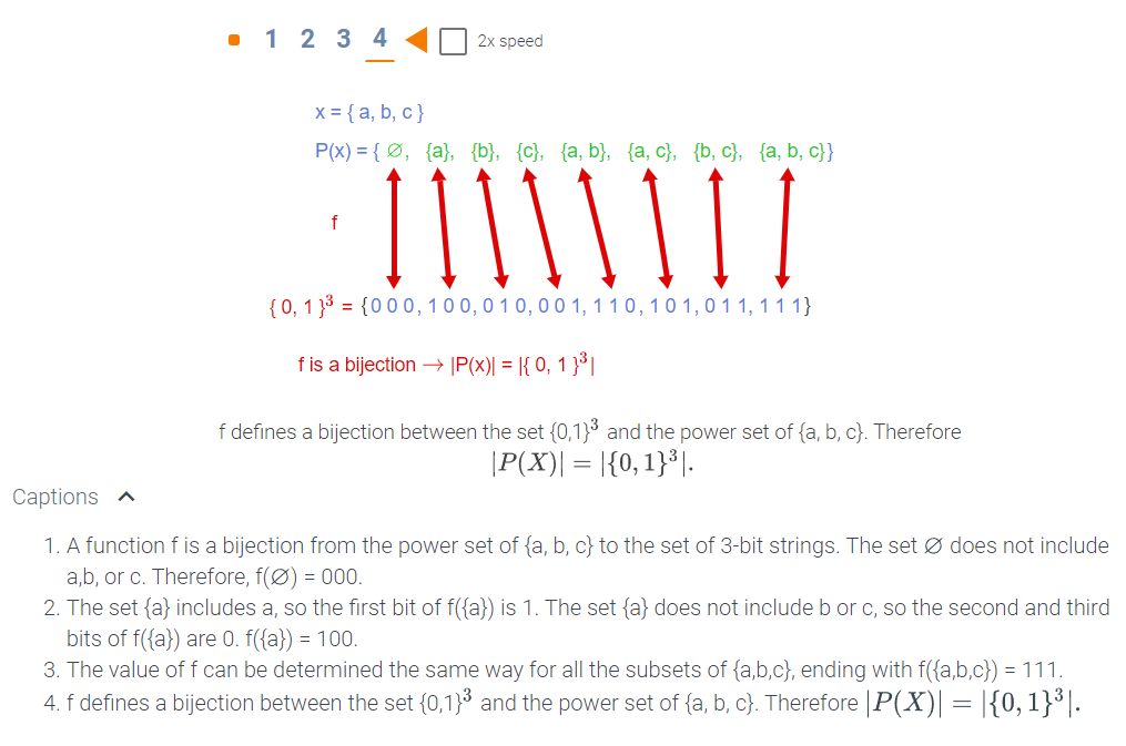
• Bijection of sets can be used to count sets. For example, creating a one-to-one correspondence between a power set, P(x), and binary strings of length n, the cardinality of the binary strings equals the cardinality of P(x).
• According to the bijection rule, bijective sets have the same cardinality.
• The bijection rule is used to count sets when there is a 1-to-1 correspondence. If there is more than a 1-to-1 correspondence (k-to-1) use the “k-to-1 rule.” To count the number of elements in a k-to-1 correspondence in the range, count the number of elements in the domain and divide by k.
  • For example, a manufacturer needs to order rubber caps for ends of their tripods. Each tripod needs 3 rubber caps. To determine the total number of rubber caps apply the k– to-1 rule using a 3-to-1 correspondence.

4.5 Lesson: The generalized product rule

Lesson introduction

In the previous lessons you learned how to count the number of possible combinations of several items using the sum and product rules. You also learned how to use the bijection and k-to-1 rules to count sets. But what if you had a situation where you had two sets with different numbers of elements in each set (different cardinalities), and you had to determine the number of possibilities for a given number of choices or steps? 

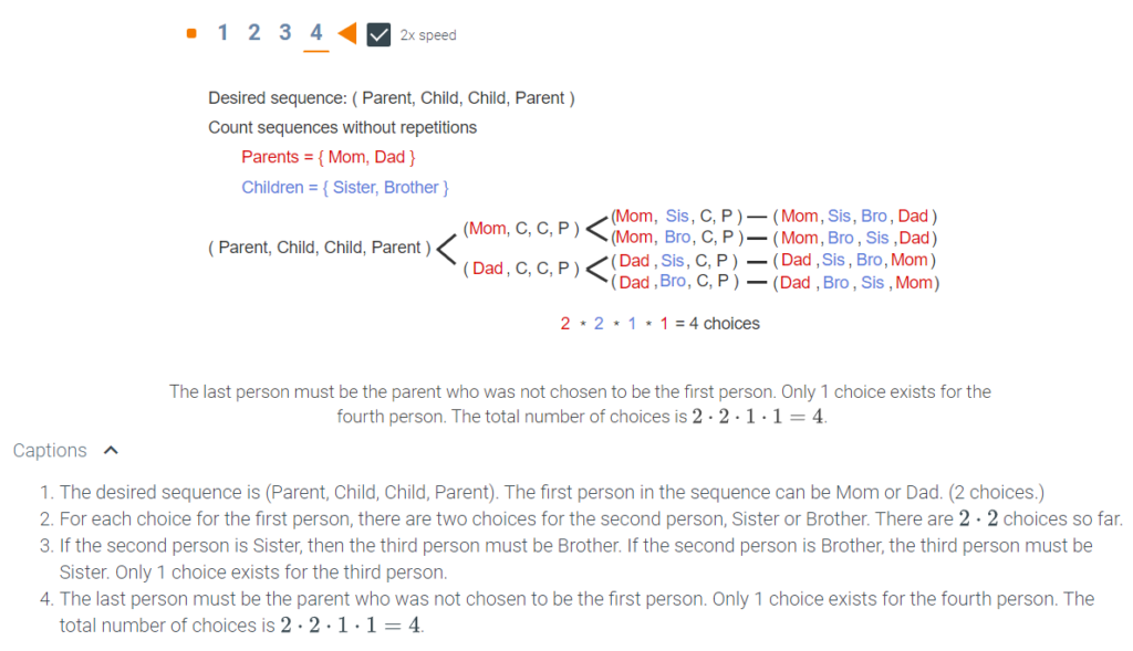
The generalized product rule says that in selecting an item from a set, if the number of choices at each step does not depend on previous choices made, then the number of items in the set is the product of the number of choices in each step.

Lesson summary

Now that you have completed this lesson you should be able to solve a counting problem using the generalized product rule. Take a moment to think about what you’ve learned in this lesson:

• The generalized product rule keeps you from having to exhaustively make lists of all possibilities when several items are being considered in several sets.
• In the generalized product rule each successive choice lowers the number of possibilities for the next choice.
• To calculate the number of possibilities using the generalized product rule, multiply the number of items for each set or step by the number in the next step, etc. In the lesson introduction there was an example with horses in a race. The number of possible outcomes is 10 x 9 x 8 = 720.
• Review this example of using the generalized product rule. Let’s say there are seven different fruit candies in one jar and four different chocolate candies in another jar. How many possibilities are there for two friends to choose two pieces of candy (one from each jar)?
  Answer: The first person has 7 x 4 choices, and the second person has 6 x 3 choices. Total number of choices = 28 x 18 = 504.

4.6 Module 14: Counting with Permutations and Combinations

This page marks the beginning of Module 14. This module contains four lessons:

• Counting permutations
• Counting subsets
• Distinguishing between subsets and permutations
• Permutations with repeating items

4.7 Lesson: Counting permutations

Lesson introduction

In the previous lessons you learned a few counting rules that applied to items in sequences and sets where the order of the items did not matter. But sometimes in counting, order does matter. In mathematics, the term “permutation” refers to a series where order does matter. For example, in a password, if the correct order is 1352, typing in 3215 will not work. 1352 and 3215 are two different permutations (or arrangements) of the digits 1, 2, 3, and 5.

Permutations

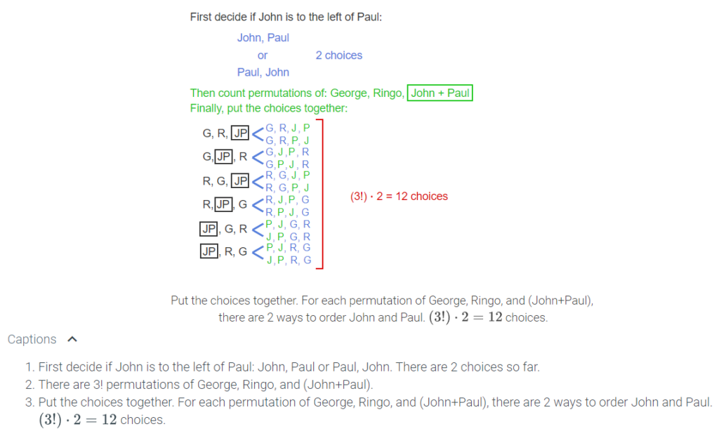
One of the most common applications of the generalized product rule is in counting permutations. An r-permutation is a sequence of r items with no repetitions, all taken from the same set. Consider the set X = {John, Paul, George, Ringo}. The sequences (Paul, Ringo, John) and (John, George, Paul) are both examples of 3-permutations over X. In a sequence, order matters, so the sequence (Paul, Ringo, John) is different from the sequence (Ringo, Paul, John). In contrast, counting subsets of objects in which order does not matter is called combinations. Care should be taken when using the term combinations when referring to the number of possibilities, because the term carries a specific meaning.

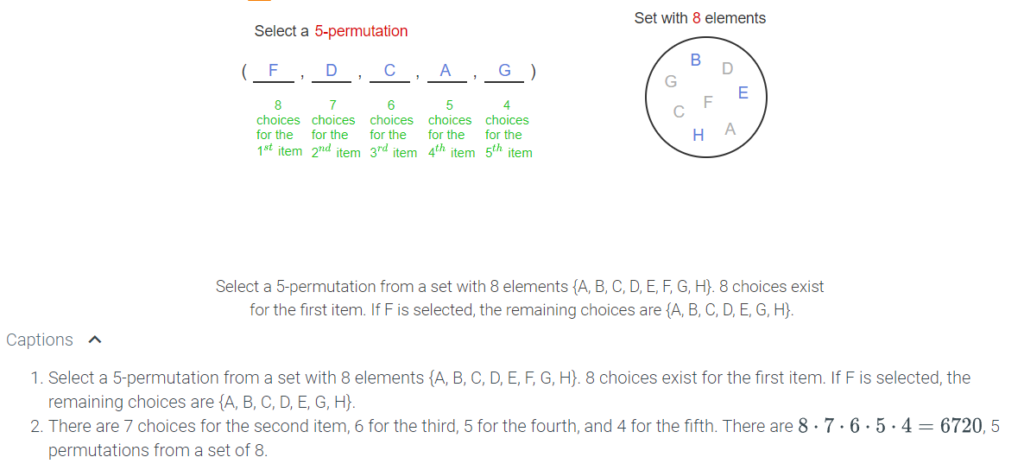
The closed form for P(n, r) is a consequence of the generalized product rule. There are n choices for the first item in the sequence because the set from which the items are drawn has n elements. Once the choice of the first item in the sequence is made, there are n – 1 choices for the next item because the first item in the sequence can not be repeated. In general, once the first i items in the sequence have been chosen, there are n – i remaining elements from which the next one can be chosen. The selection process continues until r items have been chosen for the sequence. Just before the last (r^th) item is chosen, r – 1 items have already been chosen and there are n – (r – 1) = n – r + 1 items from which to select the last item.

Lesson summary

Now that you have completed this lesson you should be able to determine the count of either r‐permutations or permutations from a set using the generalized product rule. Take a moment to think about what you’ve learned in this lesson:

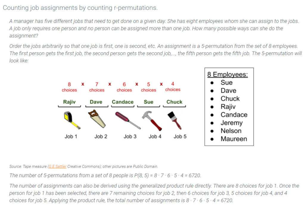
• An r-permutation is a sequence of r items with no repetitions, all taken from the same set. For example, if there are 5 permutations (r items) from a set of 8 items, the formula is P(8,5) = 8 × 7 × 6 × 5 × 4 = 6720
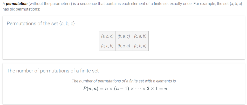
• The number of permutations (arrangements) of a finite set of items n, grouped r at a time can be calculated using factorials and, at its core, is just the generalized product rule.
• When counting the number of arrangements of a finite set, then the formula is very simply n. If there is a specified order within elements of the set, combine the elements and think of it as one element. For example, if there are 6 elements in the set, and two elements must be next to each other in the sequence, then the formula is n – 1.
• Being able to count the number of arrangements of a finite set gives a programmer the ability to determine the number of ways a set of bits, a set of ID characters, or password characters can be arranged.

4.9 Lesson: Subset and permutation examples

Lesson introduction

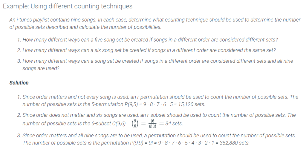
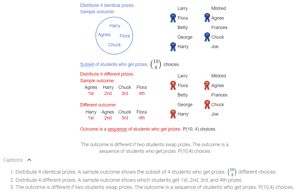
Now that you know about permutations and combinations, in this lesson you will practice distinguishing between combinations and permutations and will learn when to use each formula or procedure to count a subset. As a hint, focus on whether or not order is important!

Lesson summary

Now that you have completed this lesson you should be able to determine if a solution in a counting problem is based on subsets or permutations. Take a moment to think about what you’ve learned in this lesson:

• Use the permutation calculation if the order in which the elements of the subset are selected is important. For example, select the top four students out of ten to earn the first place, second place, third place, and fourth place prizes.
• Use the combination calculation if the order in which the elements of the subset are selected is not important. For example, select four students out of ten to earn a prize.

4.10 Lesson: Permutations with repetitions

Lesson introduction

Sometimes items in sets are not as distinct as we have assumed in every lesson to this point. Sometimes there are “look alikes”—items in a set or string that are duplicates and cannot be distinguished from each other.

This throws quite a kink into the permutation/combination counting! For example, if you are working with a string consisting of the letters in “GOOD,” there’s no way to distinguish between the two Os. There’s no way to know that {G, O} ← using the first O is different from {G, O} ← using the second O.

Permutations with repetition

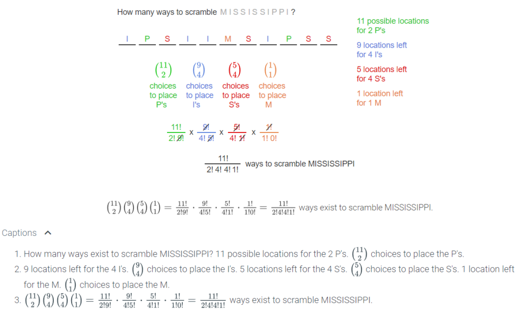
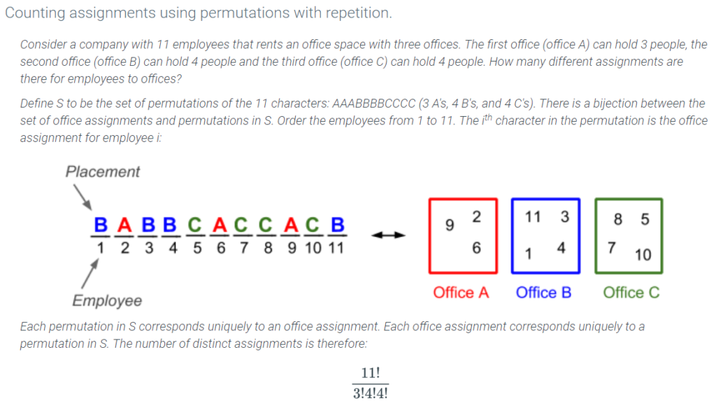
How many ways are there to scramble the letters in the word MISSISSIPPI? The question is concerned about counting different orderings which suggests counting permutations. However, a permutation is defined as an ordering of distinct objects. The letters in MISSISSIPPI have multiple repetitions: there are four S’s, four I’s, two P’s, and one M. A permutation with repetition is an ordering of a set of items in which some of the items may be identical to each other. To illustrate with a smaller example, there are 3! = 6 permutations of the letters CAT because the letters in CAT are all different. However, there are only 3 different ways to scramble the letters in DAD: ADD, DAD, DDA. The animation below shows how to count the number of distinct permutations of the letters in MISSISSIPPI by repeatedly applying the formula for counting r-subsets and putting together the choices using the product rule.

Lesson summary

Now that you have completed this lesson you should be able to determine the number of ways to permute a set with items that repeat using the formula for counting permutations with repetition. Take a moment to think about what you’ve learned in this lesson:

• In the previous lessons you worked with sets whose elements are all distinct (no repeated items). In this lesson repeated items or duplicates are being considered.
• If a string has any duplicates, simply divide by the factorial of number of times the duplicate repeats.

LEFT OFF FROM HERE – TAKING NOTES GOING FORWARD

4.12 Lesson: Counting by complement

Lesson introduction

Consider this example: you have eight cookies and three are broken; how many cookies are not broken? Well, five of course. As you may recall from the Discrete Mathematics I course, this is the concept of “counting by complement,” which most of us use all the time. You can count items or sets by complement.

As a refresher, in set theory the set and its complement together create the universal set. If the universal set is finite—which all the sets we deal with in this course are—then if you know the number of elements in the universal set and the number that are not in the set (the complement) you can calculate the number (cardinality) of the set. In other words, complements of sets are what’s left of the universal set when the elements of the original set are removed.

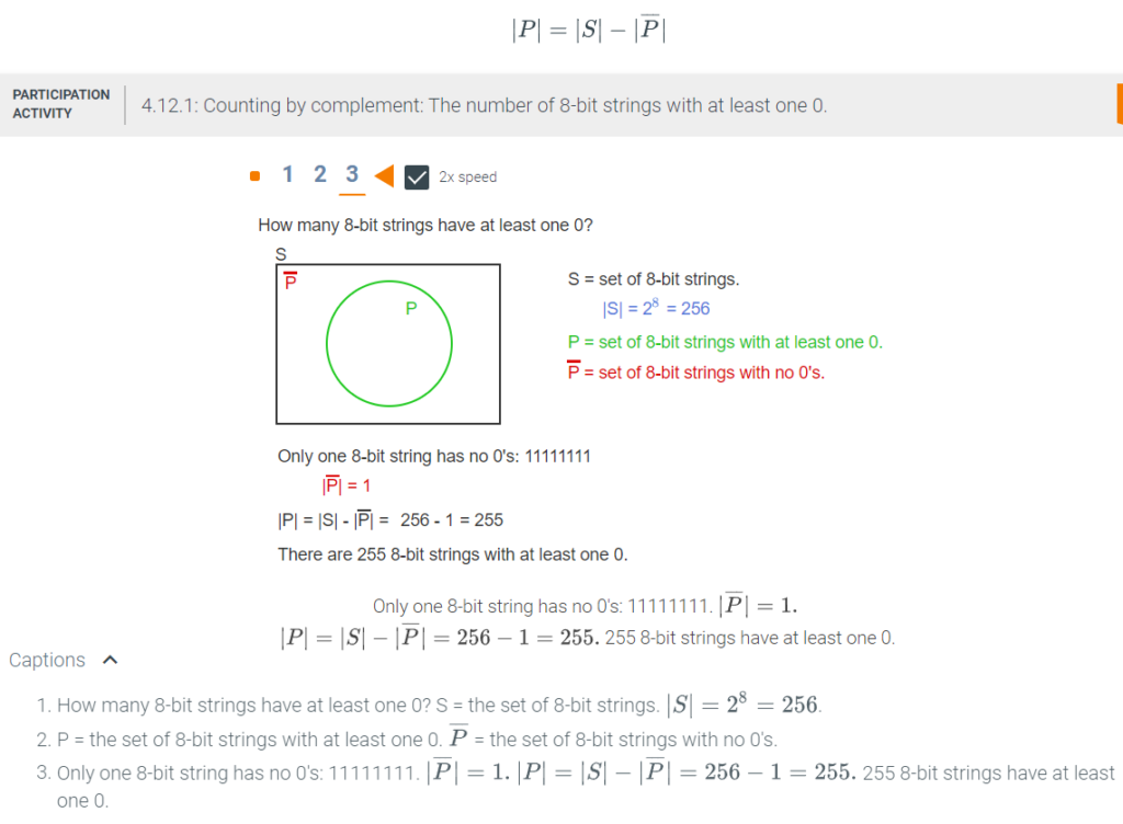
This concept is very helpful in counting “at least” or “at most” situations. For example, a coin is tossed five times. How many ways can the result have at least one tail? Since the only result without a tail is HHHHH, then it’s easier to count the compliment: number of possible outcomes after 5 tosses, is 2⁵ = 32. The complement set (no tails) has 1 element, so the number of outcomes with “at least one tail” is 32 – 1 = 31.

Counting by complement

Suppose we want to count the number of people in a room with red hair. We know that there are 20 people in the room and exactly 12 of them do not have red hair. Then we can deduce that the number of people in the room with red hair is 20 – 12 = 8. Counting by complement is a technique for counting the number of elements in a set S that have a property by counting the total number of elements in S and subtracting the number of elements in S that do not have the property. The principle of counting by complement can be written using set notation where P is the subset of elements in S that have the property.

Lesson summary

Now that you have completed this lesson you should be able to solve a counting problem relying on complements or the complement rule. Take a moment to think about what you’ve learned in this lesson:

• Counting using complements can save you a lot of time. For the purposes of this lesson, a complement set has the number of elements not in the set you are looking for.
• To count by complement:
  • Determine the number of items in your universal set
  • Subtract the cardinality of the complement from the cardinality of the universal set.
  • The result is the number of elements (cardinality) of the set you were trying to count.

4.13 Lesson: Counting multisets

Lesson introduction

As you may remember from the permutations with repetitions lesson, when you’re counting the number of arrangements of a set with duplicates, you divide the number of possible arrangements by the factorial of number of times the duplicate repeats.

In this lesson you’ll be learning about a mathematical concept called a multiset. A multiset is different from a regular set in that it can have duplicate elements where normally a set would contain distinct elements. For example, normally the regular set of letters in the word MISSISSIPPI would be {M, I, S, P}. With a multiset, the word MISSISSIPPI could have all the letters included {M, I, S, S, I, S, S, I, P, P, I}. Keep in mind, with a set, the order doesn’t matter—the braces { } indicate a set or group. The order matters in a permutation. With each arrangement of the elements, denoted with ( ), order does matter.

So multisets have duplicate elements. Why do we need them? In computer science, it’s important to be able to encode (translate or create a bijection) strings of information—messages—into another string or numerical value which the computer will understand (binary strings, for instance).

Hang on… this is a rather tough concept, but the good news is that the formula to count multisets is really easy, and is similar to the method you used to count combinations (subsets.)

Multisets

A set is a collection of distinct items. A multiset is a collection that can have multiple instances of the same kind of item. For example, {1, 2, 2, 3} is a multiset because it contains two 2’s. The curly braces denote the fact that the order in which the elements are listed does not matter, so {1, 2, 2, 3} is equal to {2, 1, 2, 3}. Multisets are useful in modeling situations in which there are several varieties of objects and one can have multiple instances of the same variety.

Suppose that a customer at a bakery is selecting a dozen cookies to buy. There are four varieties of cookies: chocolate chip, sugar, ginger, and oatmeal raisin. Cookies of the same variety are indistinguishable, so one sugar cookie is the same as any other sugar cookie. Moreover, there is a good supply of each kind, so the bakery is in no danger of running out of any of the varieties. How many ways are there to select a set of 12 cookies?

A selection of cookies is a multiset of size 12 in which the elements are cookies chosen from the four different varieties. An example of a selection of 12 cookies would be 3 chocolate chip, 2 sugar, 2 ginger, and 5 oatmeal is denoted by the multiset {C, C, C, S, S, G, G, O, O, O, O, O}.

Counting multisets

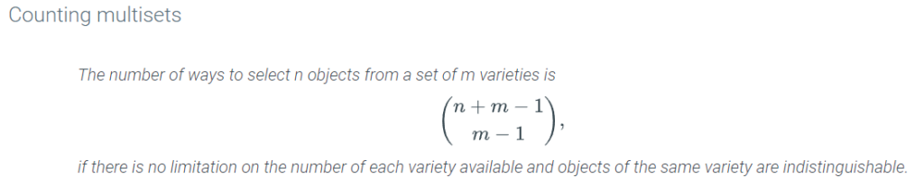
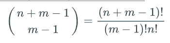
Let’s continue with the cookie example to learn how to count multisets. The formula to count multisets is

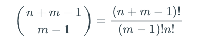
The number of objects to select is n, and the number of varieties of object is m. In the cookie example there are 12 cookies and 4 varieties, so n = 12 and m = 4. You will use the formula to determine is the number of ways to select the cookie varieties.

Before we continue, let’s look at the terms indistinguishable and distinguishable. A set of identical items are called indistinguishable because it is impossible to distinguish one of the items from another. A set of different or distinct items are called distinguishable because it is possible to distinguish one of the items from the others. This concept is important because it will help you evaluate the end result, but it does not affect the formula you will use to count multisets.

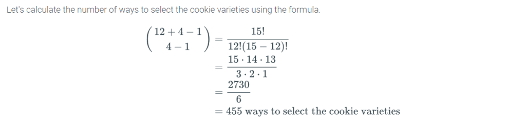
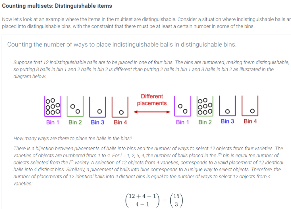
Explanation of solution (1:43)

Notice the formula you use to count the number of ways to place the balls in the bins is the same – whether or not the elements are distinguishable.

Counting multisets: Example with constraints

Let’s look at another example, except this time there is a constraint.

Suppose that a teacher distributes ten identical chocolate bars to five different kids but wants to make sure that each kid gets at least one chocolate bar. How many ways are there for the teacher distribute the chocolate bars with the additional constraint?

The constraint that each kid gets at least one chocolate bar can be satisfied by first giving a chocolate bar to each kid. Since the chocolate bars are identical, it doesn’t matter which chocolate bar goes to which kid. The figure below illustrates the situation after one chocolate bar has been given to each kid. Now there are five remaining chocolate bars to distribute. The kids are represented by bins. Giving a chocolate bar to a kid is accomplished by placing the chocolate bar in his or her bin. For the purposes of counting, distributing indistinguishable chocolate bars is the same as distributing indistinguishable balls.

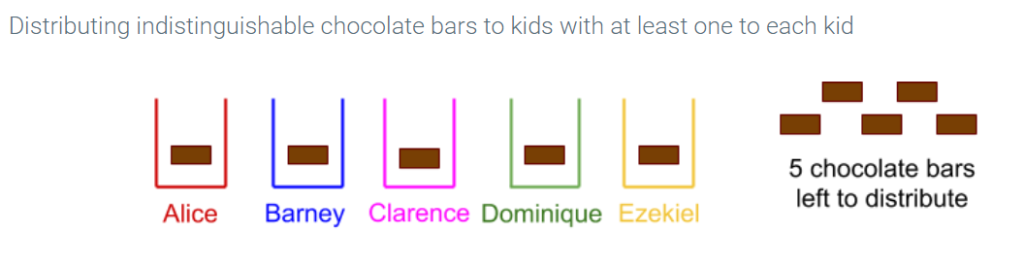
Counting the number of ways to distribute identical items to different people.

A teacher distributes ten identical chocolate bars to five different kids.

• How many ways are there for the teacher to distribute the chocolate bars among the five kids if each kid gets at least one chocolate bar?To satisfy the constraint that each kid gets at least one chocolate bar, start by giving each kid a chocolate bar. Since the chocolate bars are all the same, it does not matter who gets which one. Now there are 5 chocolate bars remaining (n = 5) to be distributed among the five kids (m = 5) and they can be distributed in any way. There are (5+5−15−1)=(94) ways to distribute the remaining chocolate bars.Explanation of solution (1:21)
• How many ways are there for the teacher to distribute the chocolate bars among the five kids if one particular kid (say Alice) gets at least two chocolate bars? (Besides the fact that Alice gets at least two chocolate bars, there are no other restrictions on how the chocolate bars are distributed).To satisfy the constraint that Alice gets at least two chocolate bars, start by giving Alice two chocolate bars. Since the chocolate bars are all the same, it does not matter which chocolate bars are given to Alice. Now there are 8 chocolate bars remaining (n = 8) to be distributed among the five kids (m = 5) which can be distributed in any way. In particular, Alice can be given more chocolate bars than the two she received initially. There are (8+5−15−1)=(124) ways to distribute the remaining chocolate bars.Explanation of solution (1:14)

Lesson summary

Now that you have completed this lesson you should be able to solve a counting problem with multisets using the complement and multiset rules. Take a moment to think about what you’ve learned in this lesson:

• Important vocabulary includes:
  • A multiset can have duplicate elements, as opposed to a regular set that has distinct elements. Multisets are very useful in applications where there are several varieties of items and at least one of those items can have multiple duplicates.
  • Distinguishable means each item/element/bit/character can be distinguished from another; each one is unique.
  • Indistinguishable means an item/element/bit/character in a set or string could repeat and you wouldn’t be able to tell them apart; they are identical duplicates.
• To calculate the number of ways to select variations (multisets) use this formula:

4.15 Lesson: Generating permutations and combinations

Lesson introduction

In the first unit of this course you learned about algorithms and how to analyze them for complexity. One of the most common types of algorithms that are evaluated for complexity are sorting algorithms. In computer science, sorting values or strings is a fundamental process to organize data. For example, bubble sorts and shell sorts are recursive algorithms for sorting processes. As the data sets get larger, so does the need for efficient sorting algorithms.

Sets of data can be sorted in lexicographic order, also known as lexical order or dictionary order. For example, think of a dictionary: the words (sets of letters) are alphabetically ordered based on the alphabetical order of their component letters. In this lesson you will first learn about the general processes to create permutations and/or combinations of sets in lexicographic order. In the following lesson, once again, counting subsets or groups in lexicographic order will be on the docket.

Before you continue, review the following terms and notations:

• n-tuple is an ordered set of n items.
• Permutations are sets, sequences, or series where order matters. Use ( ) to denote permutations.
• Combinations are subsets where order does not matter. Use { } to denote combinations

Why generate permutations and subsets

The two optimization problems described below illustrate situations in which it is necessary to generate, not just count, all the permutations of a set or subsets of a given size.

• A company has 100 employees. For every pair of people, the managers know whether those two people are compatible. The managers would like to find a group of 25 people to work together on a project such that every pair of people in the group is compatible. One approach to finding such a group is to enumerate all 25-subsets of the 100 employees and check whether everyone in the group is mutually compatible.
• A package delivery service must deliver 20 packages to 20 different locations. What is the best order to deliver the packages that minimizes the total distance traveled by the driver? One approach to finding the shortest route is to enumerate all permutations of the 20 locations and calculate the total distance traveled if the driver delivers the packages in the given order.

Lexicographic order

If A is a set of symbols or characters, n-tuples of a set A can be written without the usual punctuation (parentheses and commas) used for ordered n-tuples. For example, if A = {x, y}, the set A would be { xx, xy, yx, yy }. A sequence of characters is called a string. The set of characters used in a set of strings is called the alphabet for the set of strings..

A well-defined order imposed on the n-tuples is useful to systematically generate all the elements in a set of n-tuples. Generating the n-tuples in the set from smallest to largest ensures that each n-tuple is generated exactly once.

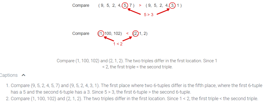
Lexicographic order is a way of ordering n-tuples in which two n-tuples are compared according to the first entry where they differ. Alphabetical order and alphanumeric order are familiar examples of lexicographic order. Words in a dictionary are ordered in lexicographic order. For example, the word “comment” appears before the word “compare” because the first place where the two words differ is the 4^th character and “m” appears before “p” in the alphabet. Although words of different lengths can be ordered lexicographically, this material only compares n-tuples of the same length.

Consider two different n-tuples, (p₁, p₂, … , p_n) and (q₁, q₂, … , q_n). To determine which n-tuple is smaller, the n-tuples are scanned from left to right to find the first index where they differ. Suppose that k is the smallest index such that p_k ≠ q_k. If p_k < q_k, then (p₁, p₂, … , p_n) < (q₁, q₂, … , q_n). Otherwise, (p₁, p₂, … , p_n) > (q₁, q₂, … , q_n).

Generating permutations in lexicographic order

A permutation of the set {1, 2, …, n} is an ordered n-tuple in which each number in {1, 2, …, n} appears exactly once. For example (2, 5, 1, 4, 3) is a permutation of the set {1, 2, 3, 4, 5}.

Any two distinct permutations over {1, 2, …, n – 1, n} can be ordered lexicographically. Generating permutations in lexicographic order is a good way to ensure that each permutation is generated exactly once. The first permutation in lexicographic order is (1, 2, …, n – 1, n) and the last permutation is (n, n – 1, …, 2, 1). The permutations of the set {1, 2, 3} are listed below in lexicographic order:

(1, 2, 3) < (1, 3, 2) < (2, 1, 3) < (2, 3, 1) < (3, 1, 2) < (3, 2, 1)

The algorithm GenLexPermutations(n) takes as input a natural number n and outputs all the permutations of {1, 2, …, n} in lexicographic order. GenLexPermutations starts with the first permutation in lexicographic order and keeps generating the next permutation until the last permutation is reached. The algorithm NextPerm(P) (described below) takes as input a permutation P and returns the smallest permutation that is larger than P.

Algorithm to generate permutations in lexicographic order

GenLexPermutations(n)

Initialize P = (1, 2, …, n – 1, n)
Output P
While P ≠ (n, n – 1, …, 2, 1),
    P = NextPerm(P)
    Output P

The final step is to find an algorithm that, given a permutation P = (p₁, p₂, …, p_n), generates the permutation just after P in lexicographical order. Consider,

P = (5, 2, 4, 3, 1)

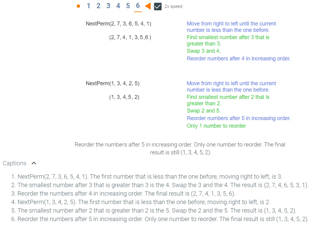
In finding the next permutation after P, some of the entries of P will be re-ordered so that the new permutation is larger but as close to P as possible. Thus the goal is to keep as much of the first part of the permutation the same. A first try might be to swap just the last two entries to get P = (5, 2, 4, 1, 3). However, since 1 < 3, the exchange results in a smaller permutation. In fact, reordering the last three entries of P in any way results in a permutation that is smaller.

The portion of P that must be re-ordered has to include the first entry where the numbers go down in scanning from right to left. In P, the first place where the numbers go down in scanning from right to left is from the 4 to the 2. Therefore, the 2 must be replaced with something larger from (…, 4, 3, 1). The smallest number that is greater than 2 in (…, 4, 3,1) is 3. So we swap 2 and 3 to get (5, 3, 4, 2, 1). Now re-order (…, 4, 2, 1) to make that portion of the permutation as small as possible, resulting in (…, 1, 2, 4) . The final result is (5, 3, 1, 2, 4).

Algorithm to generate the next permutation in lexicographic order

NextPerm(p₁, p₂, …, p_n)

Let k be the largest index such that p_k < p_k+1
    If no such k exists then (p₁, p₂, …, p_n) is the last permutation

Let j be the largest index such that p_j > p_k
Swap p_j and p_k
Reverse the order of p_k+1, …, p_n

Return( p₁, p₂, …, p_n )

Lesson summary

Now that you have completed this lesson you should be able to analyze the lexicographic order of a set using permutations. Take a moment to think about what you’ve learned in this lesson:

• An ordered set of n items can be referred to as an “n-tuple.” For example, the set of (a, b ,c, d, e) is a 5-tuple.
• Formally, lexicographical order is a way of ordering n-tuples in which two n-tuples are compared according to the first entry where they differ. Informally, lexicographical order is just sets in alphabetical order or numerical order. For example, if you were asked to put a list of books in order by the author’s last name, you would need to have an agreement on how to handle “McAllister” vs “MacAllister” or “St. John” vs “Saint Johns.” Once everyone is in agreement then you have lexicographic order.
• Review the following “algorithms” to generate permutations of sets:
  • GenLexPermutations(n) generates all the permutations of a set size n and starts with the first permutation in lexicographic order and keeps generating the next permutation until the last permutation is reached.
  • NextPerm(P) takes as input a permutation P and returns the smallest permutation that is larger than P—in other words, the “next” permutation in the lexicographic order.

4.16 Lesson: Generating r-subsets of a set

Lesson introduction

As you learned in the previous lesson there are algorithms (processes) for creating all permutations of a set in lexicographical order and to determine the next permutation in the list.

In this lesson you will take this concept one step further: create all subsets of length r in lexicographical order and determine the next subset in that order. Perhaps those subsets are names or phone numbers—this is just the beginning.

All of these processes are once again leading you toward skills needed in any type of database management at the computer science level. With an understanding of the objectives in these lessons, you will be able to create database management programs which are accurate and efficient.

Don’t worry, with practice, these skills do become easier and, after a while, become second nature to most computer science students.

Generating r-subsets of a set

Unlike sequences or n-tuples, the order in which the elements of a set or subset are written does not matter. For example, {6, 2, 8} = {2, 6, 8}. Sets can be ordered lexicographically by first sorting the elements in increasing order and then comparing the two sets as if they were ordered sequences. Consider as an example the two sets {3, 11, 2} and {6, 5, 2}. The two subsets are sorted to get {2, 3, 11} and {2, 5, 6}, and then compared as if the two sorted sets were sequences. {2, 3, 11} < {2, 5, 6} because the first element is the same in both sets but in the second element 3 < 5.

The next algorithm takes as input two natural numbers, r and n, such that r ≤ n and outputs all the r-subsets of the set {1, 2, …, n-1, n}. The elements in a subset are always listed in increasing order. The subsets are generated according to lexicographic order to ensure that each subset is generated exactly once. The first r-subset of {1, 2, …, n-1, n} in lexicographic order is {1, 2, …, r-1, r} and the last r-subset is {n-r+1, …, n-1, n}. The 3-subsets of the set {1, 2, 3, 4, 5} are listed below in lexicographic order:

{1, 2, 3} < {1, 2, 4} < {1, 2, 5} < {1, 3, 4} < {1, 3, 5} <

{1, 4, 5} < {2, 3, 4} < {2, 3, 5} < {2, 4, 5} < {3, 4, 5}

The algorithm GenLexSubsets(r, n) starts with the first r-subset in lexicographic order and keeps generating the next r-subset until the last r-subset is reached. The algorithm NextSubset(n, S) (described below) takes as input an r-subset S and natural number n and returns the smallest r-subset of {1, 2, …, n} that is larger than S.

Algorithm to generate r-subsets in lexicographic order

GenLexSubsets(r, n)

Initialize S = {1, 2, …, r-1, r}
Output S
While S ≠ {n-r+1, …, n-1, n},
    S = NextSubset(n, S)
    Output S

The final step is to find an algorithm that, given an r-subset S = {s₁, s₂, …, s_r} of {1, 2, …, n}, finds the r-subset just after S in lexicographical order. Consider,

S = {3, 5, 6, 8, 11, 12, 13},

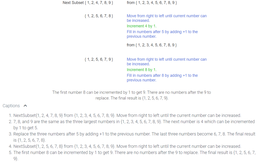
a 7-subset of {1, 2, …, 12, 13}. The goal is to change as little of the end as possible and still end up with a new r-subset that is larger than S. The last three numbers {…, 11, 12, 13} are as large as possible subject to the conditions that the numbers come from the set {1, 2, …, 12, 13}, are listed in increasing order, and are all different. Therefore, there is no way to change the last three numbers and get a 7-subset that is larger. Instead, the 8 is incremented by one, the smallest amount possible. The rest of the subset is replaced with the smallest three numbers that are all different, larger than 9, and listed in increasing order. The resulting 7-subset is {3, 5, 6, 9, 10, 11, 12}.

Algorithm to generate the next r-subset in lexicographic order

NextSubset(n, {s₁, s₂, …, s_r})

Let k be the largest index such that s_k < n – r + k
    If no such k exists then {s₁, s₂, …, s_r} is the last r-subset of {1, 2, …, n}.

s_k := s_k + 1
For j = k+1 to r
    s_j := s_j-1+1

Return( {s₁, s₂, …, s_r} )

Lesson summary

Now that you have completed this lesson you should be able to analyze the lexicographic order of an r‐subset using permutations or combinations. Take a moment to think about what you’ve learned in this lesson:

• Review the following algorithms:
  • Use GenLexSubsets(r, n) to generate a list of all subsets of length r in lexicographic order.
  • Use NextSubset(n, {s1, s2, …, sr}) to find the next subset

4.18 Lesson: Inclusion-exclusion principle

Lesson introduction

Consider this situation: You need to determine the number of ways you could draw a red card (hearts or diamonds) or a face card (king, queen, or jack) from a standard deck of cards. Initially you might be tempted to think 26 red cards plus 12 face cards equals 38 ways to select a red or face card. But that would be too many; you have inadvertently counted the red face cards twice. Since there are six red face cards in a deck, you will need to subtract six from the 38, which gives an accurate answer of 32 ways.

In your previous study on sets you learned about disjoint sets; that is, sets that have no elements in common. To count the total number of elements in sets A and B, where A and B are disjoint, you would add the cardinality of set A to set B. For example, you would use this method to determine the number ofways to draw a spade or a red card from a standard deck of cards, because elements in each set are mutually exclusive (disjoint).

However, when the sets are not disjoint—when they overlap or share some elements—simply adding cardinalities gives you a result that’s too large – as you saw in the earlier example with the red and face cards. In these cases you will need to subtract the number of elements they have in common, known as the intersection of the two sets.

In this lesson, you’ll learn all about the inclusion-exclusion principle that simply states to add the cardinality of both sets, then subtract the cardinality of the intersection if there are elements in both sets that overlap or are shared.

Inclusion and exclusion principle introduction

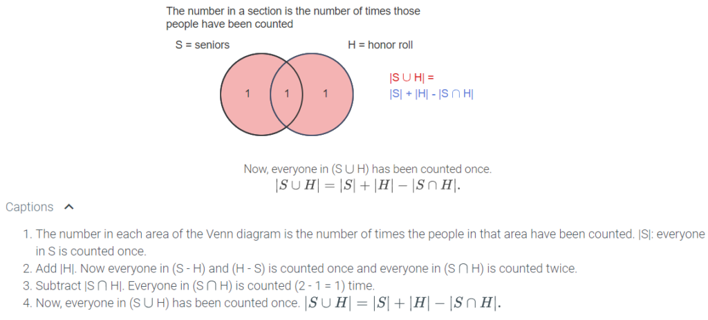
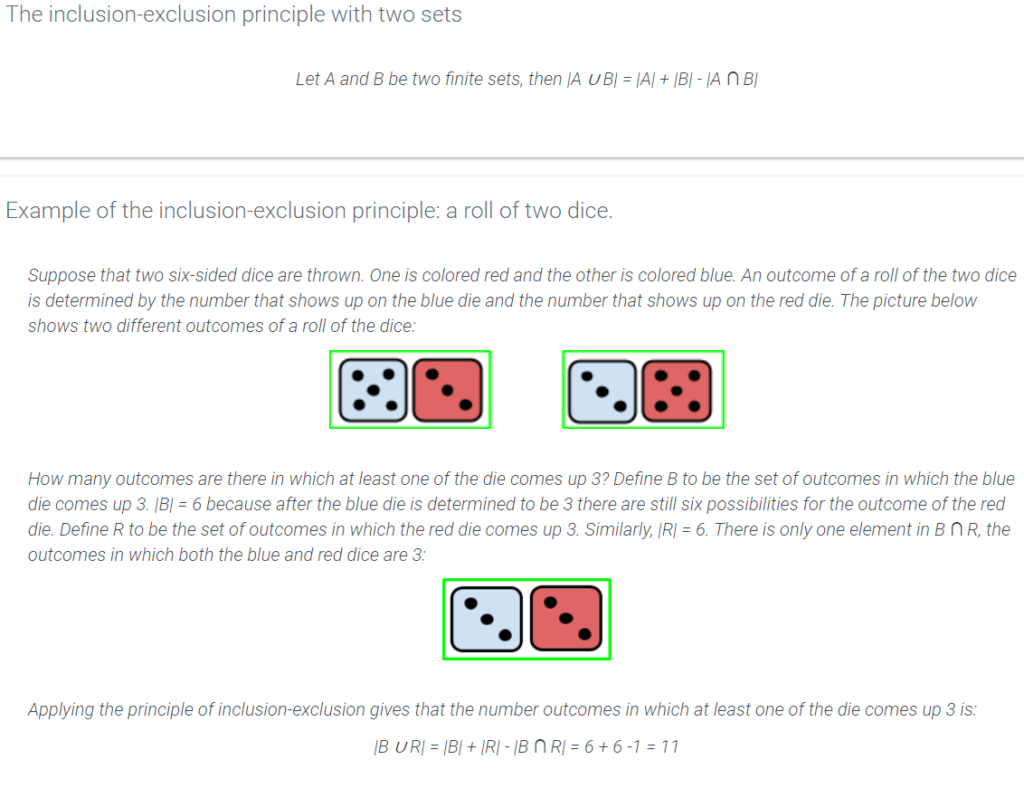
A high school gives free admission to football games to any student who is either a senior or on the honor roll. The school is trying to determine the number of students who will be admitted for free. They know the number of seniors (denoted by the variable s) as well as the number of students on the honor roll (denoted by the variable h). Is this enough information to determine the number of students eligible to attend for free? The sum (s + h) results in over counting because seniors on the honor roll are counted twice, once for being a senior and once for being on the honor roll. The school must also know the number of students who are both seniors and on the honor in order to be able to determine the number of people in either group.

Define the set S to be the set of all seniors. Define H to be the set of students on the honor roll. The school would like to count the number of students in the set S ∪ H. The principle of inclusion-exclusion is a technique for determining the cardinality of the union of sets that uses the cardinality of each individual set as well as the cardinality of their intersections. The animation below illustrates the idea with two sets:

Inclusion-exclusion with three sets

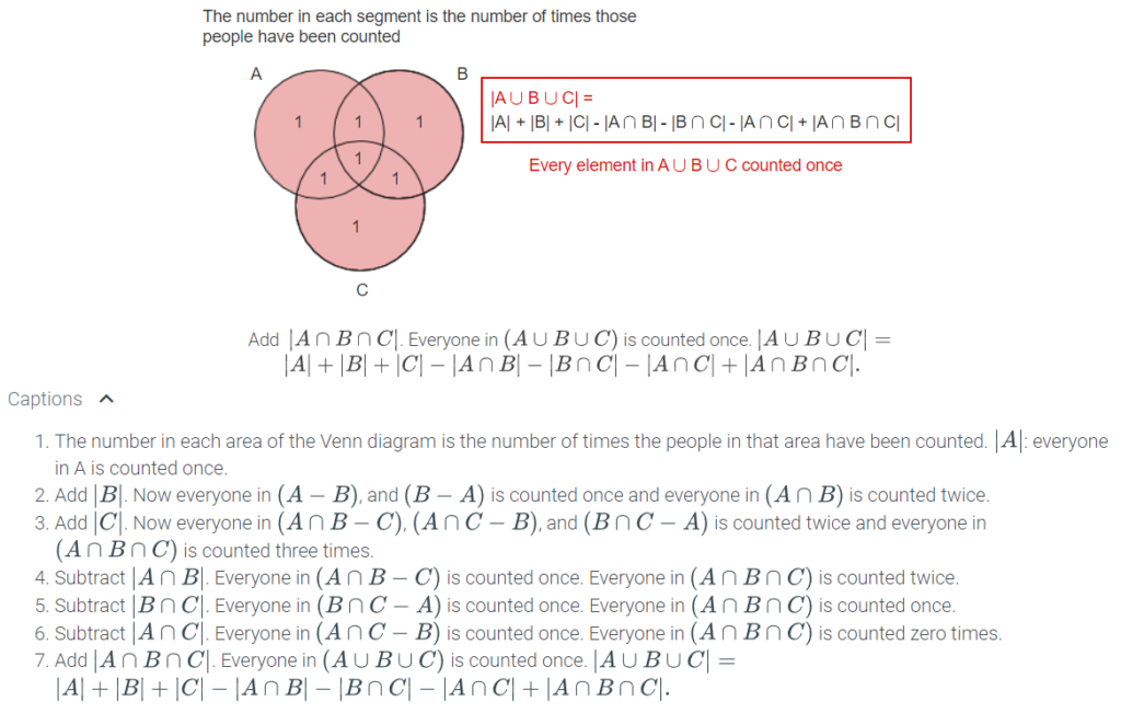
Let A, B and C be three finite sets, then

|A ∪ B ∪ C| = |A| + |B| + |C| – |A ∩ B| – |B ∩ C| – |A ∩ C| + |A ∩ B ∩ C|

The inclusion-exclusion with three sets: course enrollments.

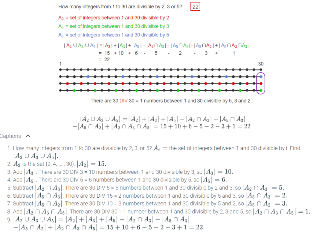
A computer science department offers three lower division classes in a given quarter: discrete math, digital logic, and introductory programming. The department would like to know the number of students enrolled in any of the three courses. Let M be the set of students enrolled in discrete math, L be the set of students enrolled in digital logic, and P the set of students enrolled in introductory programming. Here are numbers for enrollments in the courses:

• |M| = 112 students enrolled in discrete math.
• |L| = 138 students enrolled in digital logic.
• |P| = 142 students enrolled in introductory programming.
• |M ∩ L| = 25 students enrolled in both discrete math and digital logic.
• |L ∩ P| = 17 students enrolled in both digital logic and introductory programming.
• |M ∩ P| = 32 students enrolled in both introductory programming and discrete math.
• |M ∩ L ∩ P| =7 students are enrolled in all three classes.

The total number of students enrolled in any of the three courses is:

|M ∪ L ∪ P| = |M|+ |L| + |P| – |M ∩ L| – |L ∩ P| – |M ∩ P| + |M ∩ L ∩ P|

= 112 + 138 + 142 – 25 – 17 – 32 + 7 = 325

Lesson summary

Now that you have completed this lesson you should be able to solve a counting problem using the inclusion-exclusion principle. Take a moment to think about what you’ve learned in this lesson:

• When a collection of sets are disjoint—that is, mutually disjoint—counting the total number of elements is simple; just add the cardinalities.
• The inclusion-exclusion principle is applied when two or more sets intersect (are not disjoint).
• To count the total number of elements in two sets that intersect:
  • Sum the cardinalities of each set
  • Subtract the cardinality of the intersection
• To count the total number of elements in three sets, of which two intersect:
  • Sum the cardinalities of all three sets
  • Calculate the cardinality of the intersection of all three sets
  • Calculate the cardinality of the three intersections of two sets at a time
  • Subtract the cardinality of all the intersection sets
• To find the cardinality of an intersection (union) use the complement of a set.

4.19 Lesson: Binomial coefficients and combinatorial identities

Lesson introduction

Do you remember this equation from algebra: (�+�)2=(�+�)(�+�)=�2+2��+�2? It is an example of an exponentiating binomial (two-term) expression. Why is this important to you? Because you will be learning how to use the binomial theorem to count the number of ways to choose objects from a set. In programming the binomial theorem can be used in working with random variables and in statistical analysis of large data sets. At its heart, the binomial theorem is all about the patterns found when exponentiating binomial (two-term) expressions. Here’s a hint: the coefficient provides all the answers.

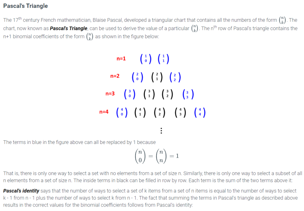
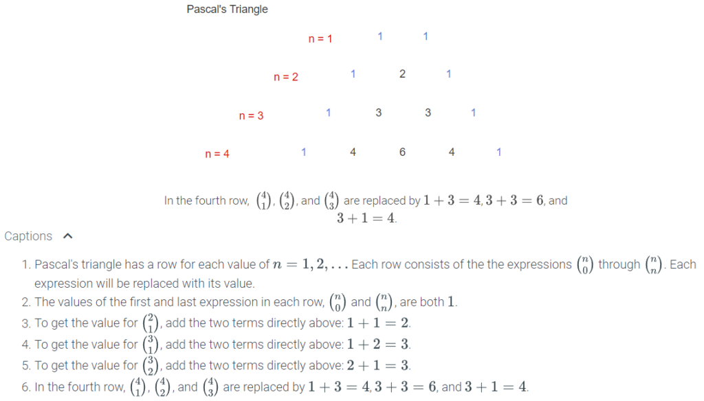
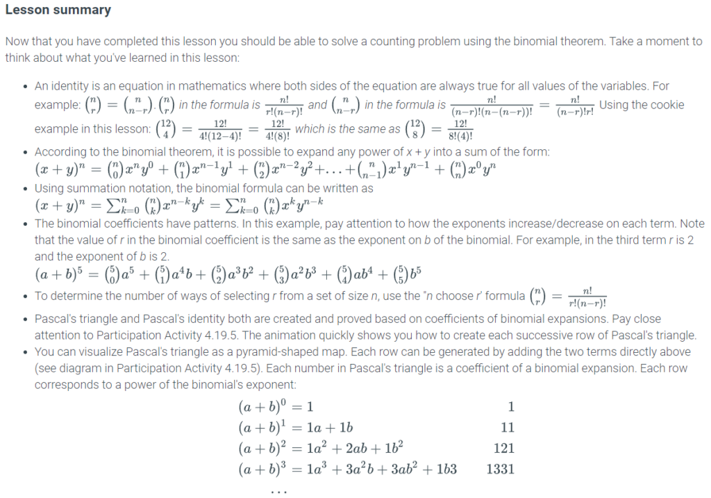
The coefficients of the binomial expansion form a pattern known as Pascal’s triangle. Once you learn the pattern, it makes expanding any exponentiation of a binomial very fast. By the way, if you find yourself intrigued by the patterns in Pascal’s triangle, know that there are a lot more which include applications involving the Fibonacci sequence, the golden ratio, and fractal geometry—just to spark your curiosity.

In this lesson you will learn how the patterns of the exponents and the coefficients can be easily calculated using the combination (subset) counting formula. Before you continue, if you need a refresher of the formula and concepts, review the Counting Subsets lesson found in Module 14.

Identities

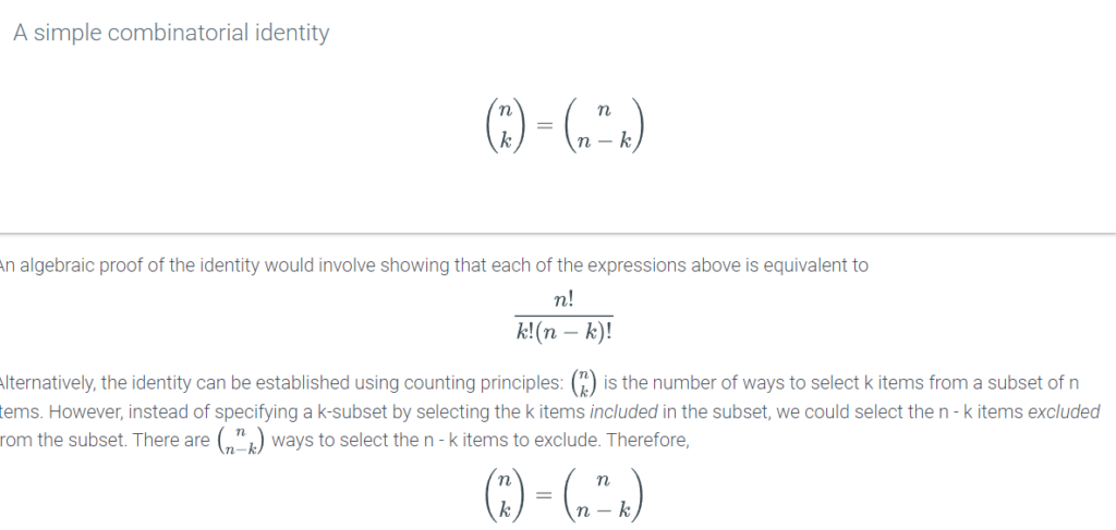
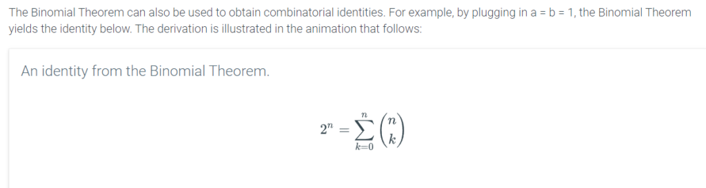
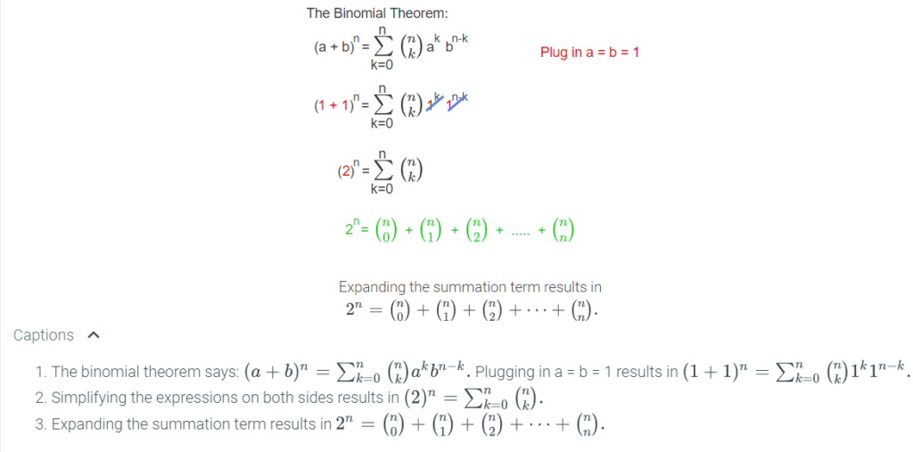
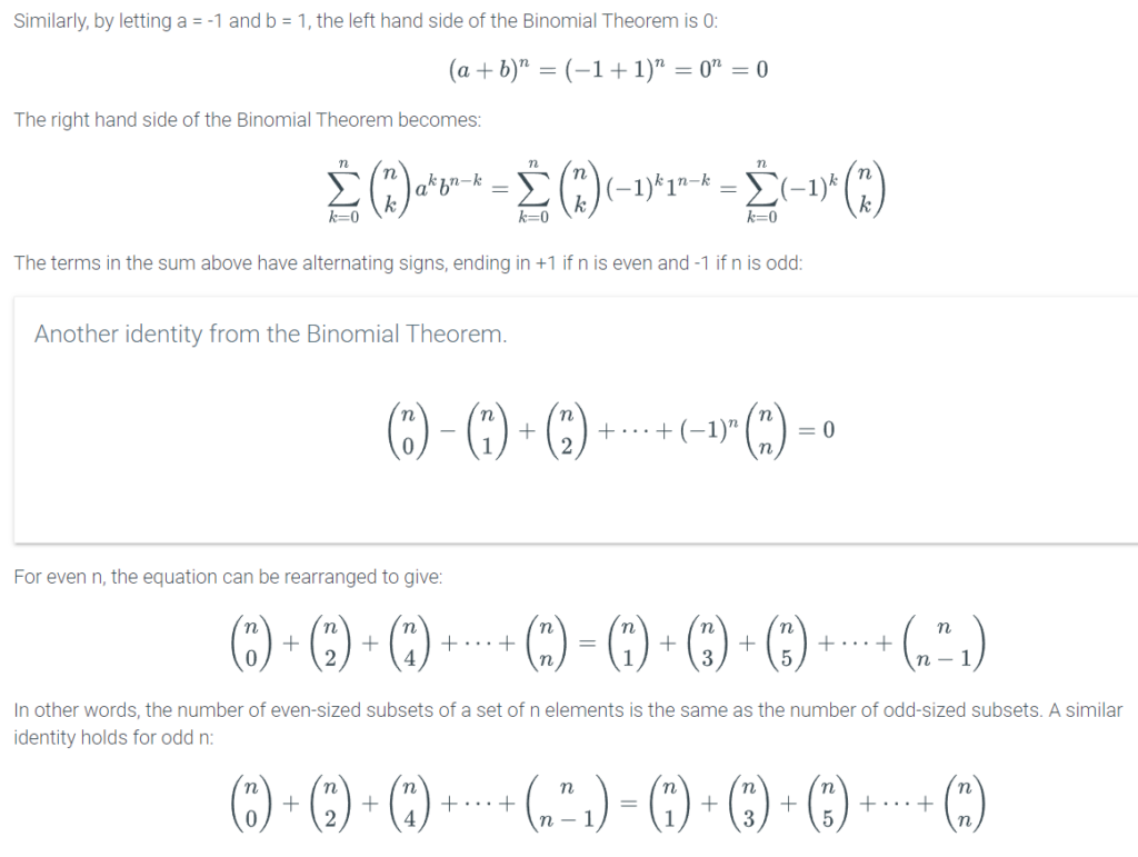
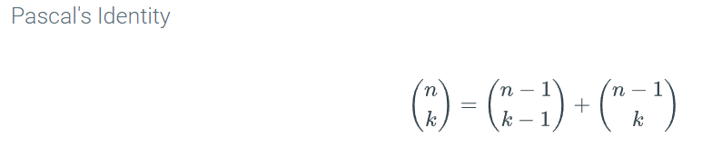
An identity is a theorem stating that two mathematical expressions are equal. An identity that involves expressions related to counting is called a combinatorial identity. Here is an example of a simple combinatorial identity:

The Binomial Theorem

The binomial (a + b)³ can be expanded to a sum of terms as follows:

(�+�)3=���+���+���+���+���+���+���+���

There is a term for every string in the set {a, b}³. Of course, since the variables a and b commute, many of these terms can be folded together. For example, aab + aba + baa = 3a²b. After collapsing all equivalent terms, the binomial can be expressed as:

(�+�)3=�3+3�2�+3��2+�3

The coefficients in the above expression are 3 and 1. (The 1 is implicitly the coefficient for the a³ and b³ terms.) The coefficients in the expansion of (a + b)ⁿ for positive integer n are called binomial coefficients.

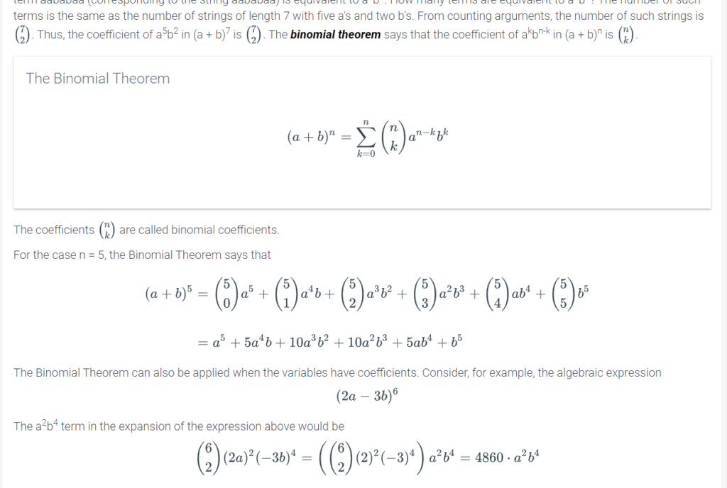
For general n, the coefficients of the terms in (a + b)³ can be expressed using ideas from counting. Notice that before coalescing common terms, there is a product of a’s and b’s for each possible string of length n over the alphabet {a, b}. For example, when n = 7, the term aababaa (corresponding to the string aababaa) is equivalent to a⁵b². How many terms are equivalent to a⁵b²? The number of such terms is the same as the number of strings of length 7 with five a’s and two b’s. From counting arguments, the number of such strings is (72). Thus, the coefficient of a⁵b² in (a + b)⁷ is (72). The binomial theorem says that the coefficient of a^kb^n-k in (a + b)ⁿ is (��).

4.20 Lesson: The pigeonhole principle

Lesson introduction

The pigeonhole principle is a surprisingly simple concept (named after its silly example of putting pigeons in boxes), yet can be used in clever ways to show functions that are not one-to-one; in other words, that there will always be a repeated value in the range of the function.

In this lesson you will see several examples of how the pigeonhole principle is used in a variety of applications. Essentially if the function has a domain with more values than the range (the target), then there is always guaranteed to be at least two values in the domain which map to the same value in the range.

Pigeonhole principle

The pigeonhole principle is a mathematical tool used to establish that repetitions are guaranteed to occur in certain sets and sequences. The pigeonhole principle says that if n+1 pigeons are placed in n boxes, then there must be at least one box with more than one pigeon. The image below shows 10 pigeons placed in 9 boxes.

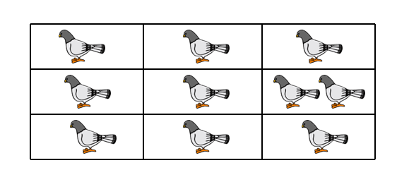
Although the principle itself appears to be obvious, it can be applied in clever ways to prove facts that are quite surprising. Below is a more mathematical version of the pigeonhole principle stated in the language of functions:

The Pigeonhole Principle

If a function f has a domain of size at least n+1 and a target of size at most n, where n is a positive integer, then there are two elements in the domain that map to the same element in the target (i.e., the function is not one-to-one).

In the mathematical statement of the pigeonhole principle, the elements of the target represent boxes and the elements of the domain represent pigeons. The function f maps the pigeons to the boxes.

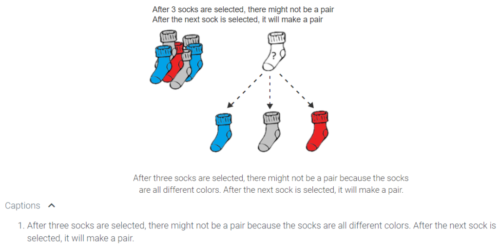
Consider a person who has a drawer filled with socks. Each sock is either blue, gray, or red. How many socks does the person have to get from their drawer before he knows that he has a pair of the same color? In this case, the domain is the set of socks picked from the drawer. The target is the set of sock colors. The function f maps a sock to its color. The pigeonhole principle says that if the socks come in three colors and four socks are selected, the person is guaranteed to have a pair of the same color. The animation below illustrates:

The generalized pigeonhole principle

Consider a function whose domain has n elements and whose target has k elements, for n and k positive integers. Then there is an element y in the target such that f maps at least ⌈�/�⌉ elements in the domain to y.

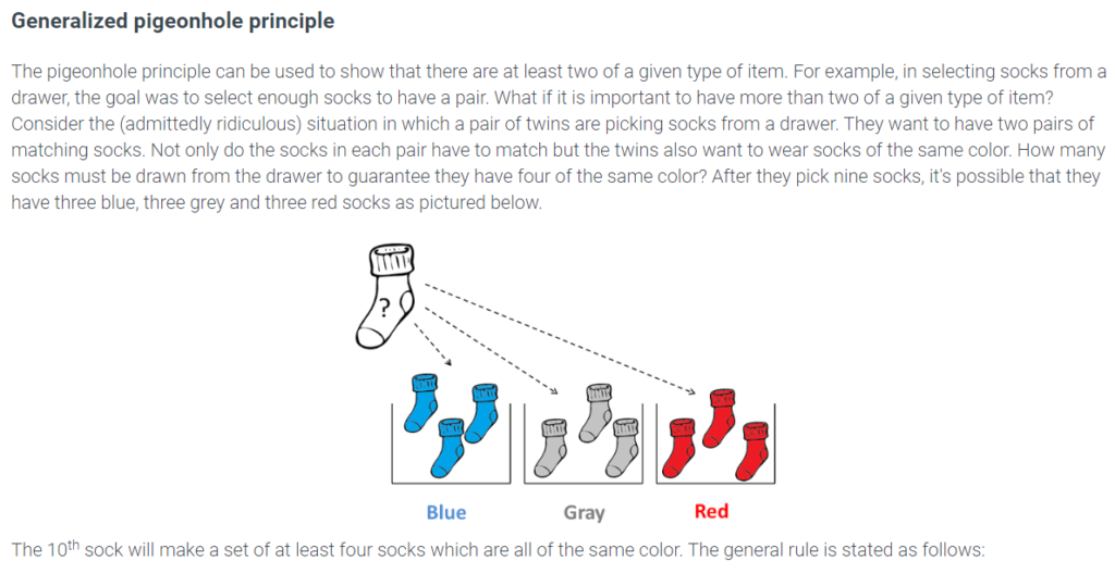
In the case of the socks, n = 10 is the number of socks and k = 3 is the number of colors. After selecting 10 socks, the twins are guaranteed that they have at least ⌈10/3⌉=4 socks which are all of the same color.

Lesson summary

Now that you have completed this lesson you should be able to solve a counting problem relying on the pigeonhole principle. Take a moment to think about what you’ve learned in this lesson:

• The pigeonhole principle is essentially stating that if a function has a domain with more values than the range (the target), then there is always guaranteed to be at least two values in the domain which map to the same value in the range. The function is not one-to-one.
  • For example, a group of 20 students is guaranteed to have several students with the same birth month. There is no way each student could have a different birth month because there are 20 students (domain) and 12 months (values in the range).
• The “contrapositive” of the principal is nicely demonstrated in 4.20.5 and again in 4.20.6. The purpose of these examples is to show you an application of why it is important to know how many items are in the domain in order to guarantee a mapping to the target.